【神经网络与深度学习-TensorFlow实践】-中国大学MOOC课程（六）（Matplotlib数据可视化））

最新推荐文章于 2021-12-20 00:12:51 发布

踏破万里无云

最新推荐文章于 2021-12-20 00:12:51 发布

阅读量732

点赞数 2

分类专栏：深度学习文章标签： tensorflow 深度学习神经网络

本文链接：https://blog.csdn.net/qq_45954434/article/details/121112686

版权

深度学习专栏收录该内容

17 篇文章 10 订阅

订阅专栏

【神经网络与深度学习-TensorFlow实践】-中国大学MOOC课程（六）（Matplotlib数据可视化

6 Matplotlib数据可视化

6 Matplotlib数据可视化

6.1 Matplotlib绘图基础

数据可视化

数据分析阶段：理解和洞察数据之间的关系；
算法调试阶段：发现问题，优化算法；
项目总结阶段：展示项目成果

Matplotlib：绘制图标的第三方库，可以快速方便地生成高质量的图标

直方图
柱形图
散点图
气泡图
折线图
三维图

6.2 安装Matplotlib库

Anaconda：安装了anaconda之后，Matplotlib就已经被安装好了
pip安装

pip install matplotlib

6.3 导入Matplotlib库中的pyplot字库

import matplotlib.pyplot as plt

6.4 Figure对象

6.4.1 创建Figure对象

figure(num,figsize,dpi,facecolor,edgecolor,frameon)

num：图形编号/名称，取值为数字/字符串；作为编号取值为数字；作为名称取值为字符串
figsize：绘图对象的宽和高，单位为英寸
dpi：绘图对象的分辨率，缺省值为80
facecolor：背景颜色
edgecolor：边框颜色
frameon：表示是否显示边框

例如：

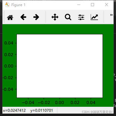
>>> import matplotlib.pyplot as plt
>>> plt.figure(figsize=(3,2),facecolor="green")#绘制一个尺寸为3*2英寸，背景为绿色的空白图形
#使用figure函数只是创建了一个画布，然后需要在这一个画布上绘制图形
<Figure size 300x200 with 0 Axes>
>>> plt.plot()#绘制一个空白图形
[]
>>> plt.show()#一定要使用show函数所绘制的图形才能显示出来

输出结果为：
在这里插入图片描述

绘图中很多的颜色都是可以改变的，下面是常用的颜色

颜色	缩略字符	颜色	缩略字符
blue	b	black	k
green	g	white	w
red	r	cyan	c
yellow	y	magenta	m

6.4.2 划分子图

一个figure对象可以看作是一个画布，其中可以有多个子图
两个坐标轴围成的区域称为轴域

subplot(行数,列数,子图序号)

对于子图序号

如果是两行一列两个字图

1
2

如果是两行两列四个子图

1	2
3	4

如果是两行三列六个字图

1	2	3
4	5	6

例如，如果把画图划分为两行两列的子图

>>> import matplotlib.pyplot as plt
>>>fig = plt.figure()
>>> plt.subplot(2,2,1)
<matplotlib.axes._subplots.AxesSubplot object at 0x000001F53EB02400>
>>> plt.subplot(2,2,2)
<matplotlib.axes._subplots.AxesSubplot object at 0x000001F5406266D8>
>>> plt.subplot(2,2,3)
<matplotlib.axes._subplots.AxesSubplot object at 0x000001F53B090908>
>>> plt.subplot(2,2,4)
<matplotlib.axes._subplots.AxesSubplot object at 0x000001F540626668>
>>> plt.show()

输出结果为：
请添加图片描述
当subplot的参数都小于10的时候，可以省略逗号

>>> import matplotlib.pyplot as plt
>>>fig = plt.figure()
>>> plt.subplot(221)
<matplotlib.axes._subplots.AxesSubplot object at 0x000001F5406A96D8>
>>> plt.subplot(222)
<matplotlib.axes._subplots.AxesSubplot object at 0x000001F53F16EA20>
>>> plt.subplot(223)
<matplotlib.axes._subplots.AxesSubplot object at 0x000001F53F16EA58>
>>> plt.subplot(224)
<matplotlib.axes._subplots.AxesSubplot object at 0x000001F53EE566A0>
>>> plt.show()

结果同上图

下面我们来看一个完整的例子：
创建一个文件first.py文件，内容如下

import matplotlib.pyplot as plt

fig = plt.figure()

plt.subplot(221)
plt.subplot(222)
plt.subplot(223)

plt.show()

在文件所在的目录下执行：

>>>python first.py

输出结果为：
请添加图片描述

6.4.3 设置中文字体

plt.rcParams["font.sans-self"]="SimHei"

rcParams：run configuration Params运行配置参数，rc参数；它们用来指定所绘制图标中的各种默认属性；是matplotlib中的全局变量；可以直接修改
font.sans-self：是字体系列
SimHei：表示中文黑体

中文字体	英文描述	中文字体	英文描述
宋体	SimSun	楷体	KaiTi
黑体	SimHei	仿宋	FangSong
微软雅黑	MicrosoftYaHei	隶书	LiSu
微软正黑体	Microsoft JhengHei	幼圆	YouYuan

rc参数被修改后，可以使用以下函数恢复标准默认配置

plt.rcdefaults()

6.4.4 添加标题

6.4.4.1 添加全局标题

suptitle(标题文字)# 这个参数是不能省略的

suptitle()函数的主要参数：

参数	说明	默认值
x	标题位置的x坐标	0.5
y	标题位置的y坐标	0.98
color	标题颜色	黑色
backgroundcolor	标题背景颜色	12
fontsize	标题的字体大小
fontweight	字体粗细	normal
fontstyle	设置字体类型
horizontalalignment	标题水平对齐方式	center
verticalaligment	标题的垂直对齐方式	top

fontsize	fontweight	fontstype	horizontalalignment	verticalaligment
xx-small	light	normal	left	center
x-small	normal	italic	right	top
small	medium	oblique	center	bottom
large	semibold			baseline
x-large	bold
xx-large	heavy
	black

6.4.4.2 添加子标题

title(标题文字)

title()函数的主要参数：

参数	说明	取值
loc	标题位置	left,right
rotation	标题文字旋转角度
color	标题颜色	黑色
fontsize	标题的字体大小
fontweight	字体粗细	normal
fontstyle	设置字体类型
horizontalalignment	标题水平对齐方式	center
verticalalignment	标题的垂直对齐方式	top
fontdict	设置参数字典

如果title()函数中要同时设置多项参数，可以使用fontdict函数把需要设置的属性都放在一个字典里，然后直接使用这个字典作为这个函数的参数

例子：

import matplotlib.pyplot as plt

plt.rcParams["font.family"] = "SimHei"#设置默认字体为中文黑体

fig = plt.figure(facecolor="lightgrey")#创建一个绘图对象，设置背景色为浅灰色

plt.subplot(221)
plt.title('子标题1')
plt.subplot(2,2,2)
plt.title('子标题2',loc="left",color="b")
plt.subplot(223)
myfontdict = {"fontsize":12,"color":"g","rotation":30}
plt.title("子标题3",fontdict=myfontdict)
plt.subplot(224)
plt.title('子标题4',color='white',backgroundcolor="black")

plt.suptitle("全局标题",fontsize=20,color="r",backgroundcolor="y")

plt.show()

执行之后得到：
请添加图片描述
结果中问题很多，全局标题盖住了第一行的子标题，第二行标题太过紧凑

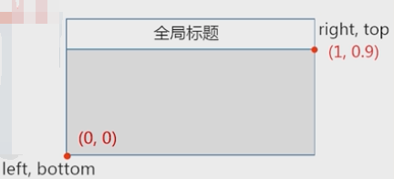
6.4.4.3 tight_layout()函数

检查坐标轴标签、刻度标签、和子图标题，自动调正子图，使之填充整个绘图区域，并消除子图之间的重叠。
使用方法：加在plt.show()函数之前
还要修改其中的rect函数

tight_layout(rect=[left,bottom.right,top])

其中四个参数如图所示，默认值是(0,0)和(1,1)
请添加图片描述
为了给全局标题留一个位置，所以取值为(0,0)和(1,0.9)

修改代码为

import matplotlib.pyplot as plt

plt.rcParams["font.family"] = "SimHei"#设置默认字体为中文黑体

fig = plt.figure(facecolor="lightgrey")#创建一个绘图对象，设置背景色为浅灰色

plt.subplot(221)
plt.title('子标题1')
plt.subplot(2,2,2)
plt.title('子标题2',loc="left",color="b")
plt.subplot(223)
myfontdict = {"fontsize":12,"color":"g","rotation":30}
plt.title("子标题3",fontdict=myfontdict)
plt.subplot(224)
plt.title('子标题4',color='white',backgroundcolor="black")

plt.suptitle("全局标题",fontsize=20,color="r",backgroundcolor="y")

plt.tight_layout(rect=[0,0,1,0.9])

plt.show()

请添加图片描述

6.2 散点图

散点图（Scatter）：是数据集点在直角坐标系中的分布图

原始数据的分布规律
数据变化的趋势

数据分组，从而观察不同数据之间的关系

6.2.1 scatter()函数绘制-散点图

scatter(x,y,scale,color,marker,label)

x,y 指明了所画的数据点的x和y坐标，不可省略，通常是python列表或者numpy数组给出所有的x和y
其他可选参数

参数	说明	默认值
x	数据点x的坐标	不可省略
y	数据点y的坐标	不可省略
scale	数据点的大小	36
color	数据点的颜色
marker	数据点的样式	‘o’(圆点)
label	图例文字

数据点样式

例子：
要求绘制出如下图

6.2.1.1 设置字体中文黑体

图中多次出现了中文，因此首先设置默认字体为中文黑体

plt.rcParams['font.sans-serif']="SimHei"

6.2.1.2 生成正态分布的x和y

标准正态分布

n = 1024
x = np.random.normal(0,1,n)
y = np.random.normal(0,1,n)

6.2.1.3 绘制散点图

绘制散点图

plt.scatter(x,y,color="blue",marker="*")

6.2.1.4 设置标题

设置标题

plt.title("标准正态分布",fontsize=20)

6.2.1.4 图右上角显示均值和方差-text()函数

设置文本

plt.text(2.5,2.5,"均 值：0\n标准差：1")

text()函数
在指定位置添加文字

text(x,y,s,fontsize,color)

参数说明：

参数	说明	默认值
x	文字的x坐标	不可省略
y	文字的y坐标	不可省略
s	显示的文字	不可省略
fontsize	文字的大小	12
color	文字的颜色	黑色

6.2.1.5 坐标轴的设置

设置坐标轴范围

plt.xlim(-4,4)
plt.ylim(-4,4)

设置坐标轴标签

plt.xlabel('横坐标x',fontsize=14)
plt.ylabel('纵坐标y',fontsize=14)#字号为14

在该程序中，坐标原点在中间，两个坐标轴都有正的和负的部分，在设置中文字体为默认字体后，坐标轴上负号的显示可能会出错，设置rcParam将axes.unicode_minus设置成False

plt.rcParams["axes.unicode_minus"]=Fasle

上述代码使得绘图时，plt会根据数据的分布区间自动加上坐标轴
如果想对坐标轴机型其他操作

函数	说明
xlabel(x,y,s,fontsize,color)	设置x轴标签
ylabel(x,y,s,fontsize,color)	设置y轴标签
xlin(xmin,xmax)	设置x轴坐标的范围
ylim(ymin,ymax)	设置y轴坐标的范围
tick_params(labelsize)	设置刻度文字的符号

6.2.1.6 完整程序例子

import numpy as np                  # 导入numpy库
import matplotlib.pyplot as plt     # 导入绘图库

plt.rcParams['font.sans-serif'] = "SimHei"
plt.rcParams['axes.unicode_minus'] = False

n = 1024
x = np.random.normal(0,1,n)
y = np.random.normal(0,1,n)

plt.scatter(x,y,color="blue",marker="*")

plt.title("标准正态分布",fontsize = 20)
plt.text(2.5,2.5,"均 值：0\n标准差：1")

plt.xlim(-4,4)
plt.ylim(-4,4)

plt.xlabel("横坐标x",fontsize=14)
plt.ylabel("纵坐标y",fontsize=14)

plt.show()

运行结果为：
请添加图片描述

6.2.1.7 增加均匀分布的点

很简单，直接再加入一组点就可以了，在同一个区域

...

n = 1024
x1 = np.random.normal(0,1,n)
y1 = np.random.normal(0,1,n)

x2 = np.random.uniform(-4,4,(1,n))
y2 = np.random.uniform(-4,4,(1,n))

plt.scatter(x1,y1,color="blue",marker="*")
plt.scatter(x2,y2,color="yellow",marker="o")

...

运行结果为：
请添加图片描述

6.2.1.8 增加图例- 区分两种点

scatter(x,y,scale,color,marker,label)
legend(loc,fontsize)

只需要在scatter中的label参数指定图例内容，然后再使用legend函数显示图例
fontsize是字体的大小，可以省略
loc参数指定图例的位置，默认为0，其取值如下：

取值	图例位置	取值	图例位置
0	best（自动寻找最优位置）	6	center left
1	upper right（右上角）	7	center right
2	upper left（左上角）	8	lower center
3	lower left	9	upper center
4	lower right	10	center
5	right

...
y2 = np.random.uniform(-4,4,(1,n))

plt.scatter(x1,y1,color="blue",marker="*",label="正态分布")
plt.scatter(x2,y2,color="yellow",marker="o",label="均匀分布")

plt.legend()
plt.title("标准正态分布",fontsize = 20)


plt.xlim(-4,4)
...

输出结果为：
请添加图片描述

6.2.1.9 最终程序

import numpy as np                  # 导入numpy库
import matplotlib.pyplot as plt     # 导入绘图库

plt.rcParams['font.sans-serif'] = "SimHei"
plt.rcParams['axes.unicode_minus'] = False

n = 1024
x1 = np.random.normal(0,1,n)
y1 = np.random.normal(0,1,n)

x2 = np.random.uniform(-4,4,(1,n))
y2 = np.random.uniform(-4,4,(1,n))

plt.scatter(x1,y1,color="blue",marker="*",label="正态分布")
plt.scatter(x2,y2,color="yellow",marker="o",label="均匀分布")

plt.legend()
plt.title("标准正态分布",fontsize = 20)


plt.xlim(-4,4)
plt.ylim(-4,4)

plt.xlabel("横坐标x",fontsize=14)
plt.ylabel("纵坐标y",fontsize=14)

plt.show()

6.3 折线图和柱形图

6.3.1 折线图

折线图（Line Chart）：散点图的基础上，将相邻的点用线段相连接

描述变量变化的趋势

6.3.1.1 绘制折线图

6.3.1.1.1 plot()函数

plot(x,y,color,marker,label,linewidth,markersize)

参数	说明	默认值
x	数据点的x坐标	0,1,2,…
y	数据点的y坐标	不可省略
color	数据点的颜色
marker	数据点的样式	‘o’
label	图例文字
linewidth	折现的宽度
markersize	数据点的大小

坐标点有python列表和numpy数组给出
color、marker、linewidth用法与散点图用法相同
除了y坐标都是可以省略的

6.3.1.2 例子

绘制这样一个折线图
请添加图片描述

6.3.1.2.1 生成随机数列

n = 24
y1 = np.random.randint(27,37,n)#温度
y2 = np.random.randint(40,60,n)#湿度

6.3.1.2.2 绘制折线图

plt.plot(y1,label='温度')
plt.plot(y2,label='湿度')

6.3.1.2.3 完整代码

import matplotlib.pyplot as plt
import numpy as np

plt.rcParams['font.sans-serif'] = "SimHei"

n = 24
y1 = np.random.randint(27,37,n)
y2 = np.random.randint(40,60,n)

plt.plot(y1,label="温度")
plt.plot(y2,label="湿度")

plt.xlim(0,23)
plt.ylim(20,70)
plt.xlabel('小时',fontsize=12)
plt.ylabel('测量值',fontsize=12)

plt.title('24小时温度湿度统计',fontsize=16)

plt.legend()
plt.show()

输出结果为:
请添加图片描述

6.3.2 柱状图

柱状图（Bar Chart）：由一系列高度不等的柱形条纹表示数据分布的情况

6.3.2.1 绘制柱状图

bar(left,height,width,facecolor,edgecolor,label)

left：就是x轴的位置序列；不可省略
height：y轴的数值序列；不可省略

请添加图片描述

width：为柱形条纹的宽度，省略时默认0.8
facecolor：柱形条纹的填充色
edgecolor：柱形条纹的边缘颜色
label：图例文字

6.3.2.2 绘制柱状图例子

请添加图片描述

6.3.2.2.1 条纹高度

y1 = [32,25,16,30,24,45,40,33,28,17,24,20]
y2 = [-23,-35,-26,-35,-45,-43,-35,-32,-23,-17,-22,-28]

6.3.2.2.2 条纹left坐标

plt.bar(range(len(y1)),y1,width=0.8,facecolor='green',edgecolor='white',label='统计量1')
plt.bar(range(len(y2)),y2,width=0.8,facecolor='red',edgecolor='white',label='统计量2')

第一个条纹的坐标是0
最后一个条纹的坐标是11

6.3.2.2.3 完整的程序

import matplotlib.pyplot as plt
import numpy as np

plt.rcParams['font.sans-serif'] = "SimHei"
plt.rcParams['axes.unicode_minus'] = False

y1 = [32,25,16,30,24,45,40,33,28,17,24,20]
y2 = [-23,-35,-26,-35,-45,-43,-35,-32,-23,-17,-22,-28]

plt.bar(range(len(y1)),y1,width=0.8,facecolor='green',edgecolor='white',label='统计量1')
plt.bar(range(len(y2)),y2,width=0.8,facecolor='red',edgecolor='white',label='统计量2')

plt.title("柱状图",fontsize=20)

plt.legend()
plt.show()

输出结果为
请添加图片描述

6.4 实例：波士顿房价数据集可视化

6.4.1 波士顿房屋数据集

6.4.1.1 Keras库

是一个高层的神经网络和深度学习库
由python编写，可以快速搭建神经网络模型，非常易于调式和扩展
TensorFlow1.4之后，成为官方API
在TensorFlow2.0，成为构架和训练模型的核心API
内置了一些常用的公共数据集，可以通过keras.detasets模块加载和访问
Keras中集成的数据集

6.4.1.1.1 波士顿房价数据集

卡内基梅隆大学，Statlib库，1978年
涵盖了麻省波士顿的506个不同郊区的房屋数据
404条训练数据集，102条测试数据集
每条数据14个字段，包含13个属性，和1个房价的平均值

6.4.1.2 使用波士顿房价数据集

6.4.1.2.1 加载数据集

可以直接使用Keras中的datasets模块访问数据集
这个数据集完整的前缀是

tensorflow.keras.datasets.boston_housing

tensorflow.keras.datasets是前缀
boston_housing是数据集名称
tensorflow.keras是keras API在tensorflow中的实现

为了简化编程，首先应当起一个简单的名字

import tensorflow as tf
boston_housing = tf.keras.datasets.boston_housing

(train_x,train_y),(test_x,test_y) = boston_housing.load_data()
# 由于该数据集，包括房屋属性和房价，而且分为训练集和测试集，所以需要4个numpy数组分别接受
# (train_x,train_y)=(训练集属性、训练集房价)
# (test_x,test_y) = (测试集属性、测试集房价)

如果你在Vscode中运行该代码报错ModuleNotFoundError: No module named 'tensorflow'，这有可能是因为VScode和anaconda没有建立链接导致，不如看看这篇文章【环境配置】在Vscode终端中使用Anaconda3中配置的环境

如果是第一次加载该数据集，会提示数据集下载提示，显示下载地址和进度
如果是windows系统下，这个数据集下载后，会自动保存在本地默认路径

C:\Users\user_name\.keras\datasets\boston_housing.npz
# user_name是当前用户的用户名
# 如果是使用管理员登陆，这里就是Administrator文件夹
# 文件保存的名称为boston_housing.npz，npz是一种压缩文件格式，主要用来存储数据
# 也可以通过其他渠道下载好这个数据集，把它保存在该文件夹下

下面使用len函数看一下数据集的条数

>>> print("Training set:", len(train_x)) 
Training set: 404
>>> print("Txsting set:", len(test_x))    
Txsting set: 102

这是默认的划分，如果想改变请看下节

6.4.1.2.2 改变数据集划分比例

import tensorflow as tf
boston_housing = tf.keras.datasets.boston_housing

(train_x,train_y),(test_x,test_y) = boston_housing.load_data(test_split=0)
# test_split是设置测试数据在整个数据中的比例，默认是0.2

然后就可以看到

>>> print("Training set:", len(train_x)) 
Training set: 506
>>> print("Txsting set:", len(test_x))    
Txsting set: 0

6.4.1.2.3 访问数据集中的数据

>>> type(train_x) 
<class 'numpy.ndarray'>
>>> type(train_y) 
<class 'numpy.ndarray'>
>>> print("Dim of train_X:",train_x.ndim) 
Dim of train_X: 2
>>> print("Shape of train_X:",train_x.shape) 
Shape of train_X: (506, 13)
>>> print("Dim of train_y:",train_y.ndim)    
Dim of train_y: 1
>>> print("Shape of train_y:",train_y.shape) 
Shape of train_y: (506,)

可以使用numpy数组中的索引和切片访问其中的数据

例如：输入train_x中的前5行数据

>>> print(train_x[:5,]) 
[[1.23247e+00 0.00000e+00 8.14000e+00 0.00000e+00 5.38000e-01 6.14200e+00
  9.17000e+01 3.97690e+00 4.00000e+00 3.07000e+02 2.10000e+01 3.96900e+02 
  1.87200e+01]
 [2.17700e-02 8.25000e+01 2.03000e+00 0.00000e+00 4.15000e-01 7.61000e+00 
  1.57000e+01 6.27000e+00 2.00000e+00 3.48000e+02 1.47000e+01 3.95380e+02 
  3.11000e+00]
 [4.89822e+00 0.00000e+00 1.81000e+01 0.00000e+00 6.31000e-01 4.97000e+00 
  1.00000e+02 1.33250e+00 2.40000e+01 6.66000e+02 2.02000e+01 3.75520e+02 
  3.26000e+00]
 [3.96100e-02 0.00000e+00 5.19000e+00 0.00000e+00 5.15000e-01 6.03700e+00 
  3.45000e+01 5.98530e+00 5.00000e+00 2.24000e+02 2.02000e+01 3.96900e+02 
  8.01000e+00]
 [3.69311e+00 0.00000e+00 1.81000e+01 0.00000e+00 7.13000e-01 6.37600e+00 
  8.84000e+01 2.56710e+00 2.40000e+01 6.66000e+02 2.02000e+01 3.91430e+02 
  1.46500e+01]]

例如：输入train_x中的某一列数据

>>> print(train_x[:,5]) 
[6.142 7.61  4.97  6.037 6.376 5.708 5.536 5.468 5.628 5.019 6.404 4.628
 5.572 6.251 5.613 5.957 7.016 6.345 6.162 6.727 6.202 6.595 7.135 6.575  
...
 5.813 7.185 6.63  6.343 8.297 6.758 6.421 6.98  6.471 6.852 6.019  
 6.376 6.108 6.417 6.209 5.093 5.987 6.395 6.957 6.229 5.414 6.495 6.009  
 5.885 6.375 6.968 4.88  5.981 7.52  5.593 6.485 5.705 6.172 6.229 5.951  
 6.593 7.061 6.03  5.884 6.897 8.259 6.812 6.122 7.333 8.78  6.273 7.802  
 6.951 6.101]

其中有506个数值，分别是每条数据中的平均房间数

6.4.2 波士顿房价数据集可视化

6.4.2.1 房间数与房价的散点图

平均房间数与房价之间的关系

#首先导入绘图库和numpy库
import tensorflow as tf
import matplotlib.pyplot as plt
import numpy as np

# 然后加载数据集
boston_housing = tf.keras.datasets.boston_housing
(train_x,train_y),(_,_) = boston_housing.load_data(test_split=0)

plt.figure(figsize=(5,5))#绘图对象的尺寸，宽和高都是5英寸
plt.scatter(train_x[:,5],train_y)# 然后绘制散点
plt.xlabel("RM")
plt.ylabel("Price($1000's)")#坐标轴标签
plt.xlim(2,10)
plt.ylim(0,60)
plt.title("5, RM-Price")#设置标题
plt.show()

输出结果为:
请添加图片描述

得出结果，屋子房间数目越多，房价越高

6.4.2.2 其他属性与房价的散点图

6.4.2.2.1 所有属性与房价的关系

import tensorflow as tf
import matplotlib.pyplot as plt
import numpy as np

boston_housing = tf.keras.datasets.boston_housing
(train_x,train_y),(test_x,test_y) = boston_housing.load_data(test_split=0)


plt.figure(figsize=(12,12))

for i in range(13):
    plt.subplot(4,4,i+1)
    plt.scatter(train_x[:,i],train_y)

plt.show()

输出结果为
在这里插入图片描述

6.4.2.2.2 添加坐标轴和标题

import tensorflow as tf
import matplotlib.pyplot as plt
import numpy as np

boston_housing = tf.keras.datasets.boston_housing
(train_x,train_y),(test_x,test_y) = boston_housing.load_data(test_split=0)

plt.rcParams['font.sans-serif'] = "SimHei"
plt.rcParams['axes.unicode_minus'] = False

titles = ["CRIM","ZN","INDUS","CHAS","NOX","RM","AGE","DIS","RAD","TAX","PTRATIO","B-1000","LSTAT","MEDV"]

plt.figure(figsize=(12,12))

for i in range(13):
    plt.subplot(4,4,i+1)
    plt.scatter(train_x[:,i],train_y)

    plt.xlabel(titles[i])
    plt.ylabel("Preice($1000's)")
    plt.title(str(i+1)+"."+titles[i]+" - Price")

plt.tight_layout(rect=[0,0,1,0.95])
plt.suptitle("各个属性与房价的关系",x = 0.5, y = 0.98,fontsize= 20)
plt.show()

输出结果为：
请添加图片描述

6.5 实例：鸢尾花数据集可视化

6.5.1 下载鸢尾花数据集

鸢尾花数据集是一个经典的用来分类的数据集
最早由Anderson测量得到，因此也被称为Anderson’s Iris Data Set数据集
1936年，就在论文中使用了它，因此也被成为统计分类的鼻祖数据集
该数据集是在加拿大的加斯帕半岛，在同一天的同一个时段，在相同的农场上，由同一个人，使用相同的测量仪器测量出来的
包括3中鸢尾花类别，每个类别有50个样本，一共150个样本；
每个样本中包括4种鸢尾花的属性特征，和鸢尾花的品种；这4种属性特征分别是花萼的长度和宽度、花瓣的长度和宽度
Iris数据集

花萼长度	花萼宽度	花瓣长度	花瓣宽度	类别标签
Sepal length	Sepal width	Petal length	Petal width	Species
				山鸢尾（Setosa）
				变色鸢尾（Versicolour）
				维吉尼亚鸢尾（Virginica）

6.5.1.1 get_file()函数-下载数据集

鸢尾花数据集不是tensorflow.keras内置集成的数据集
在使用前需要下载这些数据集，要从指定的网络地址下载数据集，可以使用以下函数

tf.keras.utils.get_file(fname,origin,cache_dir)

参数：

fname：下载后的文件名；
origin：文件的URL地址；
cache_dir：下载后文件的存储位置
windows中默认保存路径为C:\Users\\Administrator(当前用户名)\.keras\datasets

返回值：下载后的文件在本地磁盘中的绝对路径

在执行这个函数时，首先会检查要下载的文件fname是否存在，如果不存在，就根据origin参数提供的URL地址下载文件，并把它命名为fname存储在指定的目录下，并返回存储地址；如果文件已经存在，就不再下载文件，直接返回文件地址。

6.5.1.2 下载鸢尾花数据集iris

鸢尾花数据集被划分为训练数据集和测试数据集；分别放在不同的两个文件中

训练数据集文件名：iris_training.csv 120条数据
测试数据集文件名：iris_test.csv 30条数据

>>>import tensorflow as tf
>>>TRAIN_URL = "http://download.tensorflow.org/data/iris_training.csv"
>>>train_path = tf.keras.utils.get_file("iris_training.csv",TRAIN_URL)
# 第一次执行时会现在数据集
Downloading data from http://download.tensorflow.org/data/iris_training.csv
8192/2194 [================================================================================================================] - 0s 0s/step
'C:\\Users\\xxx\\.keras\\datasets\\iris_training.csv'

6.5.1.2.1 csv文件

可以使用记事本打开，也可以使用excel打开
第一行120表示一共有120行数据，数据从第2行开始到121行，所有数据都有5列，其中前4列是鸢尾花的属性，第5列是鸢尾花的种类；
用整数0，1，2分别表示山鸢尾（Setosa）、变色鸢尾（Versicolour）、维吉尼亚鸢尾（Virginica）

6.5.1.2.2 split()函数

为了提高代码的通用性，还可以使用split()函数直接从URL中获取文件名
split()函数：通过指定的分隔符对字符串进行切片一个列表。

>>> TRAIN_URL = "http://download.tensorflow.org/data/iris_training.csv"
>>> TRAIN_URL.split('/') 
['http:', '', 'download.tensorflow.org', 'data', 'iris_training.csv']
# 五个元素，两个连续的//之间是一个空的字符串

>>> fname_list = TRAIN_URL.split('/') 
>>> fname_list[-1] 
'iris_training.csv'

或者

>>> TRAIN_URL = "http://download.tensorflow.org/data/iris_training.csv"
>>> TRAIN_URL.split('/')[-1] 
'iris_training.csv'

6.5.1.3 get_file()下载数据集的通用版本

只需要改变第一行的URL即可

>>> TRAIN_URL = "http://download.tensorflow.org/data/iris_training.csv"   
>>> train_path = tf.keras.utils.get_file(TRAIN_URL.split('/')[-1],TRAIN_URL)

6.5.2 Pandas访问csv数据集

6.5.2.1 Panda库

Panda名称来自于Panel Data & Data Analysis
用于数据统计和分析的第三方库
可以高效、方便地操作大型数据集
在Anaconda中已经自带了Panda库

6.5.2.2 导入Panda库

import pandas as pd

6.5.2.3 读取csv数据集文件

6.5.2.3.1 read_csv()方法读取csv格式的文件

pd.read_csv(filepath_or_buffer,header,names)

参数filepath_or_buffer：是文件名；可以是绝对路径，也可以是相对路径；
a、在上节中，我们已经将鸢尾花数据集下载到了本地磁盘中，这里可以是绝对路径'C:\\Users\\xxx\\.keras\\datasets\\iris_training.csv'
b、如果没有下载，使用get_file()函数下载之后，返回值就是数据集在本地磁盘中的绝对路径，可以将其直接作为参数
c、从pd.read_csv()函数返回的数据类型为pandas.core.frame.DataFrame；这是二维数据表类型，是Pandas中非常常用的一种数据类型
d、参数header和names可以省略

>>> TRAIN_URL = "http://download.tensorflow.org/data/iris_training.csv"   
>>> train_path = tf.keras.utils.get_file(TRAIN_URL.split('/')[-1],TRAIN_URL)
>>> import pandas as pd
>>> pd.read_csv(train_path) 
     120    4  setosa  versicolor  virginica
0    6.4  2.8     5.6         2.2          2
1    5.0  2.3     3.3         1.0          1
2    4.9  2.5     4.5         1.7          2
3    4.9  3.1     1.5         0.1          0
4    5.7  3.8     1.7         0.3          0
..   ...  ...     ...         ...        ...
115  5.5  2.6     4.4         1.2          1
116  5.7  3.0     4.2         1.2          1
117  4.4  2.9     1.4         0.2          0
118  4.8  3.0     1.4         0.1          0
119  5.5  2.4     3.7         1.0          1

[120 rows x 5 columns]


>>> df_iris = pd.read_csv(train_path) 
>>> type(df_iris) 
<class 'pandas.core.frame.DataFrame'>

6.5.2.3.2 设置列标题（表头）-header

pd.read_csv(filepath_or_buffer,header,names)

使用header参数指定数据表中的某一行或者某几行作为列标题，header的取值是行号
默认header=0，第一行数据作为列标题（默认设置）
如果header=None，就是没有列标题

>>> TRAIN_URL = "http://download.tensorflow.org/data/iris_training.csv"   
>>> train_path = tf.keras.utils.get_file(TRAIN_URL.split('/')[-1],TRAIN_URL)
>>> df_iris = pd.read_csv(train_path) 

>>> df_iris = pd.read_csv(train_path,header=0) 
>>> df_iris.head() # 使用DataFrame对象的head()方法，输出二维表格中的前五行
# 可以看到，数据集中的第一行数据被当作列标题，但是在这里这一行数据并不是列标题，因此我们应当把数据设置为none
   120    4  setosa  versicolor  virginica
0  6.4  2.8     5.6         2.2          2
1  5.0  2.3     3.3         1.0          1
2  4.9  2.5     4.5         1.7          2
3  4.9  3.1     1.5         0.1          0
4  5.7  3.8     1.7         0.3          0


# 在这里，应当把header设置为none，数据没有表头，但是第一行显示不是所需要的数据，不对，这一行既不是样本也不是标题
>>> df_iris = pd.read_csv(train_path,header=None) 
>>> df_iris.head()
       0    1       2           3          4
0  120.0  4.0  setosa  versicolor  virginica
1    6.4  2.8     5.6         2.2          2
2    5.0  2.3     3.3         1.0          1
3    4.9  2.5     4.5         1.7          2
4    4.9  3.1     1.5         0.1          0

6.5.2.3.3 自定义列标题-names参数

names参数：自定义标题，代替header参数指定的列标题

pd.read_csv(filepath_or_buffer,header,names)

*在这里就是希望自定义个一个标题，并且不显示第一行的内容

首先，使用header=0，把第1行作为列标题
然后，设置names参数，指定新的列标题

>>> TRAIN_URL = "http://download.tensorflow.org/data/iris_training.csv"   
>>> train_path = tf.keras.utils.get_file(TRAIN_URL.split('/')[-1],TRAIN_URL)
>>> df_iris = pd.read_csv(train_path) 

>>> COLUMN_NAMES = ['SepalLength', 'SePalWidth', 'PetalLength', 'PetalWidth', 'Species']
>>> df_iris = pd.read_csv(train_path, names=COLUMN_NAMES,header=0) 
>>> df_iris.head()
   SepalLength  SePalWidth  PetalLength  PetalWidth  Species
0          6.4         2.8          5.6         2.2        2
1          5.0         2.3          3.3         1.0        1
2          4.9         2.5          4.5         1.7        2
3          4.9         3.1          1.5         0.1        0
4          5.7         3.8          1.7         0.3        0

6.5.2.3 访问数据

6.5.2.3.1 df.head()方法，前面数据

head()函数：参数为空时，默认读取二维数据表中的前5行数据
可以有参数n，表示读取前n行数据，读取8行数据

df.head(n)# 读取前n行数据

>>> df_iris.head(8) 
   SepalLength  SePalWidth  PetalLength  PetalWidth  Species
0          6.4         2.8          5.6         2.2        2
1          5.0         2.3          3.3         1.0        1
2          4.9         2.5          4.5         1.7        2
3          4.9         3.1          1.5         0.1        0
4          5.7         3.8          1.7         0.3        0
5          4.4         3.2          1.3         0.2        0
6          5.4         3.4          1.5         0.4        0
7          6.9         3.1          5.1         2.3        2

6.5.2.3.2 df.tail()方法，后面数据

tail()函数：读取后n行数据

df.tail(n)

>>> df_iris.tail(8) #这表示读取鸢尾花数据的后八行数据
     SepalLength  SePalWidth  PetalLength  PetalWidth  Species
112          5.0         3.0          1.6         0.2        0
113          6.3         3.3          6.0         2.5        2
114          5.0         3.5          1.6         0.6        0
115          5.5         2.6          4.4         1.2        1
116          5.7         3.0          4.2         1.2        1
117          4.4         2.9          1.4         0.2        0
118          4.8         3.0          1.4         0.1        0
119          5.5         2.4          3.7         1.0        1
>>> df_iris.tail() #参数为空时，表示读取后五行数据 
     SepalLength  SePalWidth  PetalLength  PetalWidth  Species
115          5.5         2.6          4.4         1.2        1
116          5.7         3.0          4.2         1.2        1
117          4.4         2.9          1.4         0.2        0
118          4.8         3.0          1.4         0.1        0
119          5.5         2.4          3.7         1.0        1

6.5.2.3.3 使用索引和切片

>>> df_iris[10:16] # 表示读取行号10-15的数据
    SepalLength  SePalWidth  PetalLength  PetalWidth  Species
10          5.2         2.7          3.9         1.4        1
11          6.9         3.1          4.9         1.5        1
12          5.8         4.0          1.2         0.2        0
13          5.4         3.9          1.7         0.4        0
14          7.7         3.8          6.7         2.2        2
15          6.3         3.3          4.7         1.6        1

6.5.2.3.4 describe()方法-显示统计信息

df.describe()方式：显示二维数据的统计信息
数据数据中的

count：总数
mean：平均值
std：标准差
min：最小值
25%：1/4
50%：1/5
75%：3/4
max：最大值

用来了解数据是否缺失

>>> df_iris.describe()
       SepalLength  SePalWidth  PetalLength  PetalWidth     Species
count   120.000000  120.000000   120.000000  120.000000  120.000000       
mean      5.845000    3.065000     3.739167    1.196667    1.000000       
std       0.868578    0.427156     1.822100    0.782039    0.840168       
min       4.400000    2.000000     1.000000    0.100000    0.000000       
25%       5.075000    2.800000     1.500000    0.300000    0.000000       
50%       5.800000    3.000000     4.400000    1.300000    1.000000       
75%       6.425000    3.300000     5.100000    1.800000    2.000000       
max       7.900000    4.400000     6.900000    2.500000    2.000000

6.5.2.3.5 DataFrame的常用属性：ndim、size、shape

属性	描述
ndim	数据表的维数
shape	数据表的形状
size	数据表元素的总个数

>>> df_iris.ndim
2
>>> df_iris.shape
(120, 5)
>>> df_iris.size 
600

6.5.2.3.6 转换为Numpy数组

直接使用numpy中的创建数组函数array()，将DataFrame对象作为参数

>>> import numpy as np
>>> iris = np.array(df_iris) 
>>> type(df_iris) 
<class 'pandas.core.frame.DataFrame'>
>>> type(iris)    
<class 'numpy.ndarray'>

也可以使用DataFrame对象自带的方法.values和.as_matrix()函数方法，前者可以，后者好像不可以了，应该是用的pandas版本太高或者太低导致

>>> iris = df_iris.values
>>> type(df_iris)
<class 'pandas.core.frame.DataFrame'>
>>> type(iris)                 
<class 'numpy.ndarray'>

6.5.2.3.6.1 numpu数组后的索引和切片

读取前6行数据，对iris数组的第一维切片

>>> iris[0:6]   # 对iris数组的第一维进行切片      
array([[6.4, 2.8, 5.6, 2.2, 2. ],
       [5. , 2.3, 3.3, 1. , 1. ],
       [4.9, 2.5, 4.5, 1.7, 2. ],
       [4.9, 3.1, 1.5, 0.1, 0. ],
       [5.7, 3.8, 1.7, 0.3, 0. ],
       [4.4, 3.2, 1.3, 0.2, 0. ]])

读取前6行数据的前4列，对iris数组的二维切片

>>> iris[0:6,0:4] 
array([[6.4, 2.8, 5.6, 2.2],
       [5. , 2.3, 3.3, 1. ],
       [4.9, 2.5, 4.5, 1.7],
       [4.9, 3.1, 1.5, 0.1],
       [5.7, 3.8, 1.7, 0.3],
       [4.4, 3.2, 1.3, 0.2]])

6.5.2.3.7 得到所有数据中的“鸢尾花种类”取值

>>> iris_y = iris[:,4] # 取到所有的行的第4列
>>> iris_y
array([2., 1., 2., 0., 0., 0., 0., 2., 1., 0., 1., 1., 0., 0., 2., 1., 2.,       2., 2., 0., 2., 2., 0., 2., 2., 0., 1., 2., 1., 1., 1., 1., 1., 2.,       2., 2., 2., 2., 0., 0., 2., 2., 2., 0., 0., 2., 0., 2., 0., 2., 0.,       1., 1., 0., 1., 2., 2., 2., 2., 1., 1., 2., 2., 2., 1., 2., 0., 2.,       2., 0., 0., 1., 0., 2., 2., 0., 1., 1., 1., 2., 0., 1., 1., 1., 2.,       0., 1., 1., 1., 0., 2., 1., 0., 0., 2., 0., 0., 2., 1., 0., 0., 1.,       0., 1., 0., 0., 0., 0., 1., 0., 2., 1., 0., 2., 0., 1., 1., 0., 0.,       1.])

6.5.2.4 Pandas其他功能简介

Pandas拥有丰富的数据处理函数
不仅可以处理二维数据表
还支持时间序列分析，具有非常强大的数据分析能力
可以自行拓展学习

6.5.3 鸢尾花数据集可视化

6.5.3.1 鸢尾花数据散点图（花瓣长宽）

请添加图片描述

6.5.3.1.1 绘制出无法区分类别的散点图

花瓣长度的列索引值是2


>>> import tensorflow as tf
>>> import matplotlib.pyplot as plt
>>> import numpy as np
>>> import pandas as pd
>>>
>>> TRAIN_URL = "http://download.tensorflow.org/data/iris_training.csv"   
>>> train_path = tf.keras.utils.get_file(TRAIN_URL.split('/')[-1],TRAIN_URL)
>>> COLUMN_NAMES = ['SepalLength', 'SePalWidth', 'PetalLength', 'PetalWidth', 'Species']
>>> df_iris = pd.read_csv(train_path, names=COLUMN_NAMES,header=0) 
>>> iris = np.array(df_iris) 


>>> iris[:,2] 
array([5.6, 3.3, 4.5, 1.5, 1.7, 1.3, 1.5, 5.1, 4.4, 1.5, 3.9, 4.9, 1.2,
       1.7, 6.7, 4.7, 5.9, 6.6, 5.3, 1.5, 5.7, 5.6, 1.3, 5.6, 5.8, 1.5,
       4. , 5.1, 4.5, 5. , 4.4, 3. , 4.5, 5.5, 4.8, 5.7, 5.1, 5.1, 1.5,
       1.4, 6.4, 5.1, 5.2, 1.9, 1.6, 5. , 1.6, 6.9, 1. , 6. , 1.4, 4.4,
       4. , 1.2, 4.7, 4.8, 6.1, 5.1, 5.4, 3.5, 3.9, 5.6, 5. , 5.5, 4.5,
       6.3, 1.3, 6.1, 5.5, 1.5, 1.3, 4.6, 1.3, 6.1, 4.9, 1.5, 3.8, 4.2,
       4.5, 5.3, 1.5, 4.7, 4.6, 4.2, 5.6, 1.5, 4.8, 4.5, 5.1, 1.3, 5.2,
       4.7, 1.4, 1.5, 5.8, 1.4, 1.4, 6.7, 4.8, 1.6, 1.4, 3.3, 1.3, 4.1,
       1.6, 1.4, 1.5, 1.4, 3.6, 1.6, 4.9, 4.1, 1.6, 6. , 1.6, 4.4, 4.2,
       1.4, 1.4, 3.7])

花瓣宽度的列索引值是3

>>> iris[:,3] 
array([2.2, 1. , 1.7, 0.1, 0.3, 0.2, 0.4, 2.3, 1.4, 0.4, 1.4, 1.5, 0.2,
       0.4, 2.2, 1.6, 2.3, 2.1, 2.3, 0.4, 2.1, 2.1, 0.4, 1.4, 1.6, 0.2,
       1.2, 1.8, 1.5, 1.7, 1.3, 1.1, 1.5, 2.1, 1.8, 2.3, 2. , 2.4, 0.3,
       0.3, 2. , 1.9, 2.3, 0.4, 0.2, 1.5, 0.2, 2.3, 0.2, 1.8, 0.2, 1.4,
       1.3, 0.2, 1.4, 1.8, 1.9, 1.9, 2.3, 1. , 1.1, 2.4, 1.9, 1.8, 1.5,
       1.8, 0.2, 2.5, 1.8, 0.2, 0.2, 1.3, 0.2, 2.3, 1.8, 0.1, 1.1, 1.3,
       1.5, 1.9, 0.2, 1.4, 1.5, 1.3, 2.4, 0.1, 1.4, 1.3, 1.6, 0.3, 2. ,
       1.2, 0.3, 0.2, 2.2, 0.3, 0.2, 2. , 1.8, 0.2, 0.2, 1. , 0.3, 1. ,
       0.4, 0.2, 0.2, 0.2, 1.3, 0.2, 1.8, 1.3, 0.2, 2.5, 0.6, 1.2, 1.2,
       0.2, 0.1, 1. ])

绘制散点图

>>> plt.scatter(iris[:,2],[iris[:,3]])
<matplotlib.collections.PathCollection object at 0x00000201AA808508>
>>> plt.show()

输出结果为：
在这里插入图片描述
可以看到，虽然散点图被绘制出来了，但是不同类别的花没有区分开来

6.5.3.1.2 色彩映射

将参数c（表示点的颜色）指定为一个列表或数组，所绘制图形的颜色，可以随这个列表或数组中元素的值而变换，变换所对应的颜色由参数cmap中的颜色所提供。

plt.scatter(x,y,c,cmap)

例如：

>>> x = np.arange(10) 
>>> y = np.arange(10) 
>>> dot_color = [0,1,2,0,1,2,2,1,1,0] 
>>> plt.scatter(x,y,20,dot_color,cmap='brg')       
<matplotlib.collections.PathCollection object at 0x00000201A9E6BD08>
>>> plt.show()

运行结果为：
请添加图片描述

对于鸢尾花数据集，我们应该使用鸢尾花的种类作为颜色变化的依据

import tensorflow as tf
import matplotlib.pyplot as plt
import numpy as np
import pandas as pd

TRAIN_URL = "http://download.tensorflow.org/data/iris_training.csv"   
train_path = tf.keras.utils.get_file(TRAIN_URL.split('/')[-1],TRAIN_URL)
COLUMN_NAMES = ['SepalLength', 'SePalWidth', 'PetalLength', 'PetalWidth', 'Species']
df_iris = pd.read_csv(train_path, names=COLUMN_NAMES,header=0) 
iris = np.array(df_iris) 

plt.scatter(iris[:,2],[iris[:,3]],c=iris[:,4],cmap='brg')
plt.show()

输出结果为
请添加图片描述

6.5.3.1.3 添加标题和坐标轴标签

# 导入必要的库
import tensorflow as tf
import matplotlib.pyplot as plt
import numpy as np
import pandas as pd

# 下载数据集
TRAIN_URL = "http://download.tensorflow.org/data/iris_training.csv"   
train_path = tf.keras.utils.get_file(TRAIN_URL.split('/')[-1],TRAIN_URL)

# 定义类、标题、列表并读取数据集文件
COLUMN_NAMES = ['SepalLength', 'SePalWidth', 'PetalLength', 'PetalWidth', 'Species']
df_iris = pd.read_csv(train_path, names=COLUMN_NAMES,header=0) 

# 将Pandas二维数据表转化问numpy二维数组
iris = np.array(df_iris) 

# 绘制散点图
plt.scatter(iris[:,2],[iris[:,3]],c=iris[:,4],cmap='brg')
plt.title("Anderson's Iris Data Set\n(Bule->Setosa | Red->Versicolor | Green->Virginica)")# 添加图表题
plt.xlabel(COLUMN_NAMES[2])
plt.ylabel(COLUMN_NAMES[3])# 设置坐标轴标签
plt.show()# 显示图形

输出结果为：
在这里插入图片描述

通过花瓣的长宽可以很好的区分开鸢尾花
那么通过数据集中的其他属性是否也能够较好的区分鸢尾花种类

6.5.3.2 鸢尾花数据散点图（其他属性）

有效的组合有6种，对角线不行，对称的不需要

6.5.3.2.1 绘制第1行4个子图

先绘制第一行中的四个字图

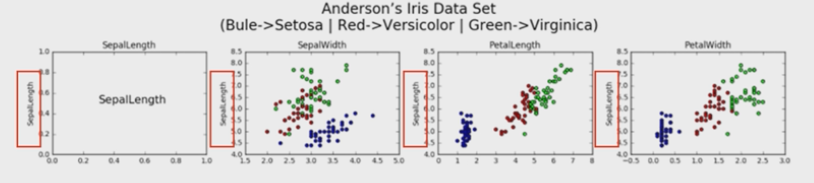
for i in range(4):
	plt.subplot(1,4,i+1)

	if(i==0):
		plt.text(0.3,0.5,COLUMN_NAMES[0],fontsize=15)
	else:
		plt.scatter(iris[:,i],iris[:,0],c=iris[:,4],cmap='brg')
		
	plt.title(COLUMN_NAMES[i])# 横坐标标签使用子图标题来实现
	plt.ylabel(COLUMN_NAMES[0])

下面是完整的代码：

import tensorflow as tf
import matplotlib.pyplot as plt
import numpy as np
import pandas as pd

TRAIN_URL = "http://download.tensorflow.org/data/iris_training.csv"   
train_path = tf.keras.utils.get_file(TRAIN_URL.split('/')[-1],TRAIN_URL)

COLUMN_NAMES = ['SepalLength', 'SePalWidth', 'PetalLength', 'PetalWidth', 'Species']
df_iris = pd.read_csv(train_path, names=COLUMN_NAMES,header=0) 

iris = np.array(df_iris) 

fig = plt.figure('Iris Data',figsize=(15,3))

fig.suptitle("Anderson's Iris Data Set\n(Bule->Setosa | Red->Versicolor | Green->Virginica)")

for i in range(4):
	plt.subplot(1,4,i+1)

	if(i==0):
		plt.text(0.3,0.5,COLUMN_NAMES[0],fontsize=15)
	else:
		plt.scatter(iris[:,i],iris[:,0],c=iris[:,4],cmap='brg')
		
	plt.title(COLUMN_NAMES[i])# 横坐标标签使用子图标题来实现
	plt.ylabel(COLUMN_NAMES[0])

plt.tight_layout(rect=[0,0,1,0.9])

plt.show()

输出结果为：
请添加图片描述

6.5.3.2.2 绘制4*4的16个子图

底层循环设为i（行）；第二层循环设为 j（列）
子图序号可以表示为：4*i + (j+1)

fig = plt.figure('Iris Data',figsize=(15,15))

fig.suptitle("Anderson's Iris Data Set\n(Bule->Setosa | Red->Versicolor | Green->Virginica)")
for i in range(4):
	for j in range(4):
		plt.subplot(4,4,4*i+(j+1))
		if(i==j):
			plt.text(0.3,0.5,COLUMN_NAMES[0],fontsize=15)
		else:
			plt.scatter(iris[:,j],iris[:,i],c=iris[:,4],cmap='brg')
			
		plt.title(COLUMN_NAMES[j])# 横坐标标签使用子图标题来实现
		plt.ylabel(COLUMN_NAMES[i])

plt.tight_layout(rect=[0,0,1,0.93])

plt.show()

完整的代码如下：

import tensorflow as tf
import matplotlib.pyplot as plt
import numpy as np
import pandas as pd

TRAIN_URL = "http://download.tensorflow.org/data/iris_training.csv"   
train_path = tf.keras.utils.get_file(TRAIN_URL.split('/')[-1],TRAIN_URL)

COLUMN_NAMES = ['SepalLength', 'SePalWidth', 'PetalLength', 'PetalWidth', 'Species']
df_iris = pd.read_csv(train_path, names=COLUMN_NAMES,header=0) 

iris = np.array(df_iris) 

fig = plt.figure('Iris Data',figsize=(15,15))

fig.suptitle("Anderson's Iris Data Set\n(Bule->Setosa | Red->Versicolor | Green->Virginica)")
for i in range(4):
	for j in range(4):
		plt.subplot(4,4,4*i+(j+1))
		if(i==j):
			plt.text(0.3,0.5,COLUMN_NAMES[0],fontsize=15)
		else:
			plt.scatter(iris[:,j],iris[:,i],c=iris[:,4],cmap='brg')
			
		plt.title(COLUMN_NAMES[j])# 横坐标标签使用子图标题来实现
		plt.ylabel(COLUMN_NAMES[i])

plt.tight_layout(rect=[0,0,1,0.93])

plt.show()

输出如下：
请添加图片描述

6.5.3.2.3 我的代码（仅修改一些参数为了图好看，大可不必来看）

上述是教程中源代码，但是我运行，子图的标题会有覆盖等等小问题，所以我改了一些参数，可以不看的

import tensorflow as tf
import matplotlib.pyplot as plt
import numpy as np
import pandas as pd

TRAIN_URL = "http://download.tensorflow.org/data/iris_training.csv"   
train_path = tf.keras.utils.get_file(TRAIN_URL.split('/')[-1],TRAIN_URL)

COLUMN_NAMES = ['SepalLength', 'SePalWidth', 'PetalLength', 'PetalWidth', 'Species']
df_iris = pd.read_csv(train_path, names=COLUMN_NAMES,header=0) 

iris = np.array(df_iris) 

fig = plt.figure('Iris Data',figsize=(12,12))

fig.suptitle("Anderson's Iris Data Set\n(Bule->Setosa | Red->Versicolor | Green->Virginica)")
for i in range(4):
	for j in range(4):
		plt.subplot(4,4,4*i+(j+1))
		if(i==j):
			plt.text(0.3,0.5,COLUMN_NAMES[0],fontsize=10)
		else:
			plt.scatter(iris[:,j],iris[:,i],8,c=iris[:,4],cmap='brg')
			
		plt.title(COLUMN_NAMES[j],fontsize=10)# 横坐标标签使用子图标题来实现
		plt.ylabel(COLUMN_NAMES[i],fontsize=10)

plt.tight_layout(rect=[0,0,1,0.98])

plt.show()

输出结果为：
请添加图片描述

6.6 参考文献

[1] 神经网络与深度学习——TensorFlow实践

踏破万里无云

关注

2
点赞
踩
11

收藏

觉得还不错? 一键收藏
0
评论
【神经网络与深度学习-TensorFlow实践】-中国大学MOOC课程（六）（Matplotlib数据可视化））

【神经网络与深度学习-TensorFlow实践】-中国大学MOOC课程（六）（Matplotlib数据可视化6 Matplotlib数据可视化6.1 Matplotlib绘图基础6.2 安装Matplotlib库6.3 导入Matplotlib库中的pyplot字库6.4 Figure对象6.4.1 创建Figure对象6.4.2 划分子图6 Matplotlib数据可视化6.1 Matplotlib绘图基础数据可视化数据分析阶段：理解和洞察数据之间的关系；算法调试阶段：发现问题，优化算法；
复制链接

扫一扫

专栏目录