Deepmd-kit 机器学习训练步骤

0 背景：略。

本文以Si作为例子讲述。

1 数据的获取。

训练数据对势函数的训练有着决定性的影响。数据集的量有500-2000不等，当然数据集越多训练的越好。除此之外还有体系的原子数，同样原子数越多训练的越好。但是也要考虑到时间成本。数据集的获取是通过VASP进行第一性的计算和运行获取。本文中通过VASP进行MD动力学过程，运行1000步，随机抽取200个数据集作为测试集，800个数据集作为训练集。

a:VASP运行需要4个文件：POSCAR，POTCAR，KPOINTS，INCAR。这些都可以用vaspkit软件自动生成，这里不过多叙述，INCAR如下：

Global Parameters
ISTART =  1            (Read existing wavefunction, if there)
ISPIN  =  1            (Non-Spin polarised DFT)
# ICHARG =  11         (Non-self-consistent: GGA/LDA band structures)
LREAL  = .FALSE.       (Projection operators: automatic)
 ENCUT  =  500        (Cut-off energy for plane wave basis set, in eV)
PREC   =  Accurate   (Precision level: Normal or Accurate, set Accurate when perform structure lattice relaxation calculation)
LWAVE  = .TRUE.        (Write WAVECAR or not)
LCHARG = .TRUE.        (Write CHGCAR or not)
ADDGRID= .TRUE.        (Increase grid, helps GGA convergence)
# LVTOT  = .TRUE.      (Write total electrostatic potential into LOCPOT or not)
# LVHAR  = .TRUE.      (Write ionic + Hartree electrostatic potential into LOCPOT or not)
# NELECT =             (No. of electrons: charged cells, be careful)
# LPLANE = .TRUE.      (Real space distribution, supercells)
# NWRITE = 2           (Medium-level output)
# KPAR   = 2           (Divides k-grid into separate groups)
# NGXF    = 300        (FFT grid mesh density for nice charge/potential plots)
# NGYF    = 300        (FFT grid mesh density for nice charge/potential plots)
# NGZF    = 300        (FFT grid mesh density for nice charge/potential plots)
 
Electronic Relaxation
ISMEAR =  0
SIGMA  =  0.05
EDIFF  =  1E-08
 
Molecular Dynamics
IBRION =  0            (Activate MD)
NSW    =  1000          (Max ionic steps)
EDIFFG = -1E-02        (Ionic convergence, eV/A)
IWAVPR = 1
POTIM  =  1            (Timestep in fs)
SMASS  =  0            (MD Algorithm: -3-microcanonical ensemble, 0-canonical ensemble)
TEBEG  =     300     (Start temperature K)
TEEND  =     300     (Final temperature K)
MDALGO =  1         (Andersen Thermostat)
# ISYM   =  0          (Switch symmetry off)
#NWRITE =  0            (For long MD-runs use NWRITE=0 or NWRITE=1)
 

b:建立三个目标文件夹：00.data  ;01.train ;02.lmp.将vasp运行的OUTCAR复制到00.data中，运行如下python代码进行数据集的划分。

import dpdata 
import numpy as np
data = dpdata.LabeledSystem('OUTCAR', fmt = 'vasp/outcar') 
print('# the data contains %d frames' % len(data))           #输出OUTCAR数据文件包含的帧数，这里从屏幕输出可以看出是200帧
index_validation = np.random.choice(1000,size=200,replace=False) #随机选取40帧作为验证数据，其余为训练数据
index_training = list(set(range(1000))-set(index_validation))    
data_training = data.sub_system(index_training)
data_validation = data.sub_system(index_validation)
data_training.to_deepmd_npy('training_data')
data_validation.to_deepmd_npy('validation_data')
print('# the training data contains %d frames' % len(data_training)) 
print('# the validation data contains %d frames' % len(data_validation)) 

2.数据的训练，设置input.json 文件如下：

{
    "_comment": " model parameters",
    "model": {
	"type_map":	["Si"],
	"descriptor" :{
	    "type":		"se_e2_a",
	    "sel":		[20],
	    "rcut_smth":	0.50,
	    "rcut":		6.00,
	    "neuron":	 [25, 50, 100],
                  "axis_neuron":	16,
	    "resnet_dt":	false,
	    "seed":		1,
	    "_comment":		" that's all"
	},
	"fitting_net" : {
	    "neuron":		[240, 240, 240],
	    "resnet_dt":	true,
	    "seed":		1,
	    "_comment":		" that's all"
	},
	"_comment":	" that's all"
    },

    "learning_rate" :{
	"type":		"exp",
	"decay_steps":	5000,
	"start_lr":	0.001,	
	"stop_lr":	3.51e-8,
	"_comment":	"that's all"
    },

    "loss" :{
	"type":		"ener",
	"start_pref_e":	0.02,
	"limit_pref_e":	1,
	"start_pref_f":	1000,
	"limit_pref_f":	1,
	"start_pref_v":	0,
	"limit_pref_v":	0,
	"_comment":	" that's all"
    },

    "training" : {
	"training_data": {
	    "systems":		["../00.data/training_data"],
	    "batch_size":	"auto",
	    "_comment":		"that's all"
	},
	"validation_data":{
	    "systems":		["../00.data/validation_data"],
	    "batch_size":	"auto",
	    "numb_btch":	1,
	    "_comment":		"that's all"
	},
	"numb_steps":	1000000,
	"seed":		10,
	"disp_file":	"lcurve.out",
	"disp_freq":	1000,
	"save_freq":	5000,
	"_comment":	"that's all"
    },    

    "_comment":		"that's all"
}

设置完之后，进行训练。dp train input.json。超算计算脚本编写可咨询我。

3.数据的冻结与压缩。

 
  冻结模型    dp freeze -o graph.pb

 
压缩模型  dp compress -i graph.pb -o graph-compress.pb

4.预测数据和测试数据的测试。

命令：dp test -m graph-compress.pb -s ../00.data/validation_data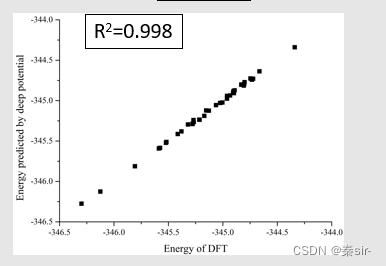

大概流程就这么多，有不清楚的地方，欢迎关注公众号：硕博科研小助手，联系我。