


 这篇博客介绍了作者基于《最优状态估计-卡尔曼,H∞及非线性滤波》一书的第11章进行的MATLAB仿真实验,涵盖H∞滤波的相关内容。通过四个示例,包括H∞滤波的界限计算、比较卡尔曼滤波与H∞滤波的性能、连续时间H∞滤波的解以及时间变量和稳态滤波的误差分析。实验结果显示H∞滤波在抑制噪声方面表现出优势。博客强调了状态估计理论在运动控制领域的应用价值,并建议读者通过实践来巩固相关知识。
《最优状态估计-卡尔曼,H∞及非线性滤波》:第11章 H∞滤波
前言
《最优状态估计-卡尔曼,H∞及非线性滤波》由国外引进的一本关于状态估计的专业书籍,2006年正式出版,作者是Dan Simon教授,来自克利夫兰州立大学,电气与计算机工程系。主要应用于运动估计与控制,学习本文的过程中需要有一定的专业基础知识打底。
本书共分为四个部分,全面介绍了最优状态估计的理论和方法。第1部分为基础知识,回顾了线性系统、概率论和随机过程相关知识,介绍了最小二乘法、维纳滤波、状态的统计特性随时间的传播过程。第2部分详细介绍了卡尔曼滤波及其等价形式,介绍了卡尔曼滤波的扩展形式,包括相关噪声和有色噪声条件下的卡尔曼滤波、稳态滤波、衰减记忆滤波和带约束的卡尔曼滤波等(掌握了卡尔曼,基本上可以说这本书掌握了一半)。第3部分详细介绍了H∞滤波,包括时域和频域的H∞滤波,混合卡尔曼/H∞滤波,带约束的H∞ 滤波。第4部分介绍非线性系统滤波方法,包括扩展卡尔曼滤波、无迹卡尔曼滤波及粒子滤波。本书适合作为最优状态估计相关课程的高年级本科生或研究生教材,或从事相关研究工作人员的参考书。
其实自己研究生期间的主研方向并不是运动控制,但自己在本科大三时参加过智能车大赛,当时是采用PID对智能车的运动进行控制,彼时凭借着自学的一知半解,侥幸拿到了奖项。到了研究生期间,实验室正好有研究平衡车的项目,虽然自己不是那个方向,但实验室经常有组内报告,所以对运动控制在实际项目中的应用也算有了基本的了解。参加工作后,有需要对运动估计与控制进行相关研究,所以接触到这本书。
这次重新捡起运动控制,是希望自己可以将这方面的知识进行巩固再学习,结合原书的习题例程进行仿真,简单记录一下这个过程。主要以各章节中习题仿真为主,这是本书的第十一章的4个仿真示例(仿真平台:32位MATLAB2015b),话不多说,开始!
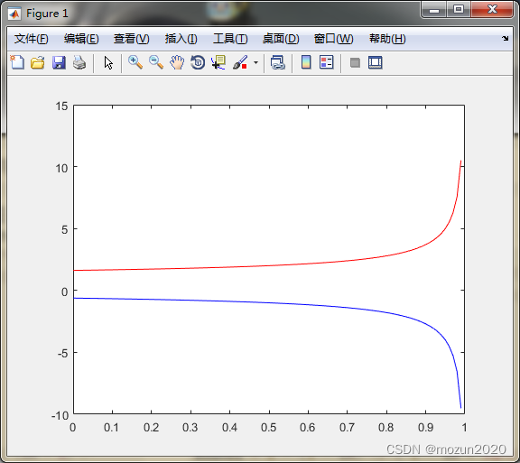
1. MATLAB仿真:示例11.2(1)
%%%%%%%%%%%%%%%%%%%%%%%%%%%%%%%%%%%%%%%%%%%%%%%%%%%%
%功能:《最优状态估计-卡尔曼,H∞及非线性滤波》示例仿真
%示例11.2: HinfEx1a.m
%环境:Win7,Matlab2015b
%Modi: C.S
%时间:2022-05-02
%%%%%%%%%%%%%%%%%%%%%%%%%%%%%%%%%%%%%%%%%%%%%%%%%%%%

function HinfEx1a

th = 0 : .01 : .99;
%th = 5 : .01 : 10;

if 1 == 1
    p1 = (1-th+sqrt((th-1).*(th-5)))/2./(1-th);
    p2 = (1-th-sqrt((th-1).*(th-5)))/2./(1-th);
    close all;
    plot(th, p1, 'r'); hold;
    plot(th, p2, 'b');
    return;
end

Bound1 = 2 * (1 - th) ./ ( 1 - th + sqrt( (th - 1) .* (th - 5) ) );
Bound2 = 2 * (1 - th) ./ ( 1 - th - sqrt( (th - 1) .* (th - 5) ) );
Limit = th - 1;

close all;
plot(th, Limit, 'k'); hold;
plot(th, Bound1, 'r');
plot(th, Bound2, 'b');
2. MATLAB仿真:示例11.2(2)
%%%%%%%%%%%%%%%%%%%%%%%%%%%%%%%%%%%%%%%%%%%%%%%%%%%%
%功能:《最优状态估计-卡尔曼,H∞及非线性滤波》示例仿真
%示例11.2: HinfEx1b.m
%环境:Win7,Matlab2015b
%Modi: C.S
%时间:2022-05-02
%%%%%%%%%%%%%%%%%%%%%%%%%%%%%%%%%%%%%%%%%%%%%%%%%%%%

function HinfEx1b(SSFlag, BiasFlag)

% Compare the Kalman and H-infinity estimators for a scalar system.
% SSFlag = 1 if the steady state estimator is used.
% BiasFlag = 1 if the process noise is biased

BiasFlag =1;%


if ~exist('SSFlag', 'var')
    SSFlag = 1;
end

if SSFlag ~= 0
    KK = (1+sqrt(5))/(3+sqrt(5));
    theta = 1/3;
    %theta = 1/10;
    PH = (1-theta+sqrt((theta-1)*(theta-5)))/2/(1-theta);
    KH = PH * inv(1 - theta * PH + PH);
end

kf = 20;
PK = 1;
PH = PK;
Q = 10;
R = 10;
x = 0;
xhatK = x + sqrt(PK); % Kalman filter estimate (in error by one sigma)
xhatH = xhatK; % H-infinity estimate
xArr = [x];
xhatKArr = [xhatK];
xhatHArr = [xhatH];
for k = 1 : kf
    y = x + sqrt(R) * randn;
    if SSFlag == 0
        KK = PK * inv(1 + PK) * R;
        PK = PK * inv(1 + PK) + Q;
        KH = PH * inv(1 - PH/2 + PH) * R;
        PH = PH * inv(1 - PH/2 + PH) + Q;
    end
    x = x + sqrt(Q) * randn;
    if BiasFlag
        x = x + 10;
    end
    xhatK = xhatK + KK * (y - xhatK);
    xhatH = xhatH + KH * (y - xhatH);
    xArr = [xArr x];
    xhatKArr = [xhatKArr xhatK];
    xhatHArr = [xhatHArr xhatH];
end

k = 0 : kf;
close all;
figure; hold on;
plot(k, xArr, 'k', 'LineWidth', 2.5);
plot(k, xhatKArr, 'r--', k, xhatHArr, 'b:');
set(gca,'FontSize',12); set(gcf,'Color','White');
legend('true state', 'Kalman estimate', 'H_{\infty} estimate');
xlabel('time'); ylabel('state value');
set(gca,'box','on');

RMSK = sqrt(norm(xArr-xhatKArr)^2/(kf+1));
RMSH = sqrt(norm(xArr-xhatHArr)^2/(kf+1));
disp(['Kalman RMS estimation error = ', num2str(RMSK)]);
disp(['H-infinity RMS estimation error = ', num2str(RMSH)]);
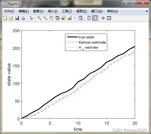
>> HinfEx1b
Kalman RMS estimation error = 14.2754
H-infinity RMS estimation error = 10.768
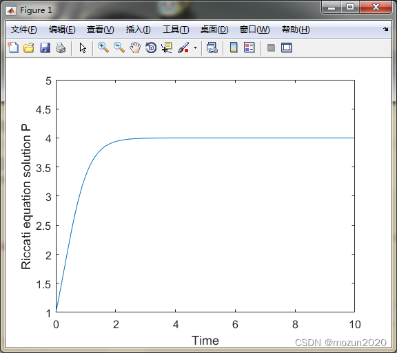
3. MATLAB仿真:示例11.3(1)
%%%%%%%%%%%%%%%%%%%%%%%%%%%%%%%%%%%%%%%%%%%%%%%%%%%%
%功能:《最优状态估计-卡尔曼,H∞及非线性滤波》示例仿真
%示例11.3: HinfContEx1a.m
%环境:Win7,Matlab2015b
%Modi: C.S
%时间:2022-05-02
%%%%%%%%%%%%%%%%%%%%%%%%%%%%%%%%%%%%%%%%%%%%%%%%%%%%

function HinfContEx1a

% Continuous time H-infinity filtering example, theta = 7/16

P0 = 1;
c = (9*P0+4)/(40*P0-160);
t = 0 : 0.01 : 10;
P = (4 + 160 * c * exp(5*t/2)) ./ (-9 + 40 * c * exp(5*t/2));

close all;
plot(t,P);
set(gca,'FontSize',12); set(gcf,'Color','White');
xlabel('Time'); ylabel('Riccati equation solution P');
axis([0 10 1 5]);
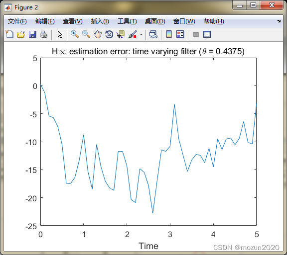
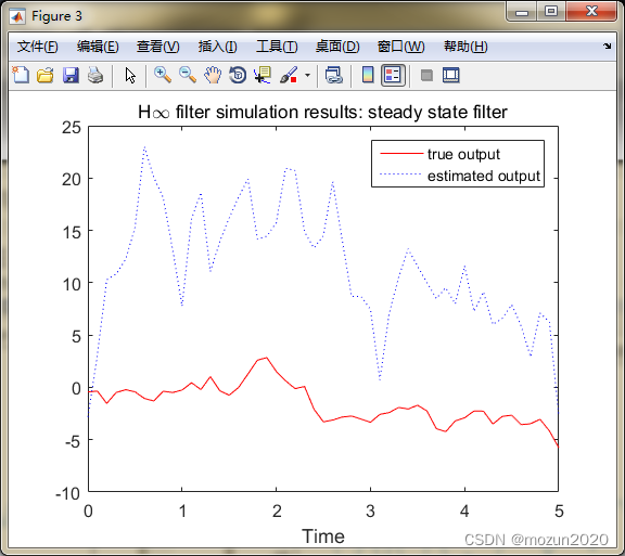
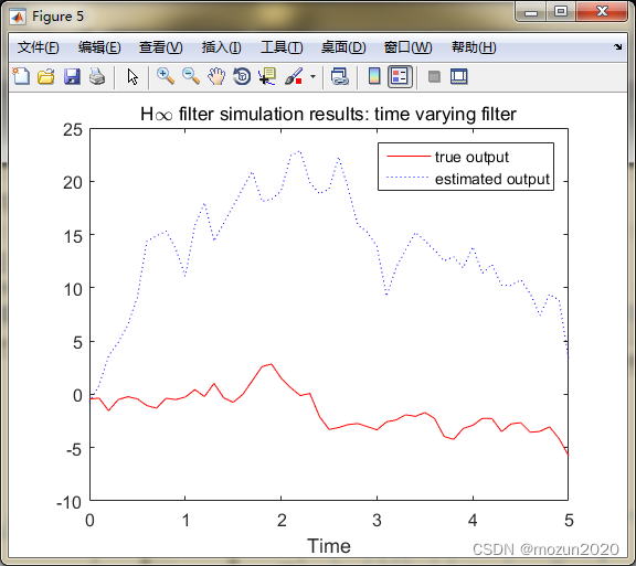
4. MATLAB仿真:示例11.3(2)
%%%%%%%%%%%%%%%%%%%%%%%%%%%%%%%%%%%%%%%%%%%%%%%%%%%%
%功能:《最优状态估计-卡尔曼,H∞及非线性滤波》示例仿真
%示例11.3: HinfContEx1b.m
%环境:Win7,Matlab2015b
%Modi: C.S
%时间:2022-05-02
%%%%%%%%%%%%%%%%%%%%%%%%%%%%%%%%%%%%%%%%%%%%%%%%%%%%
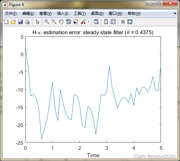
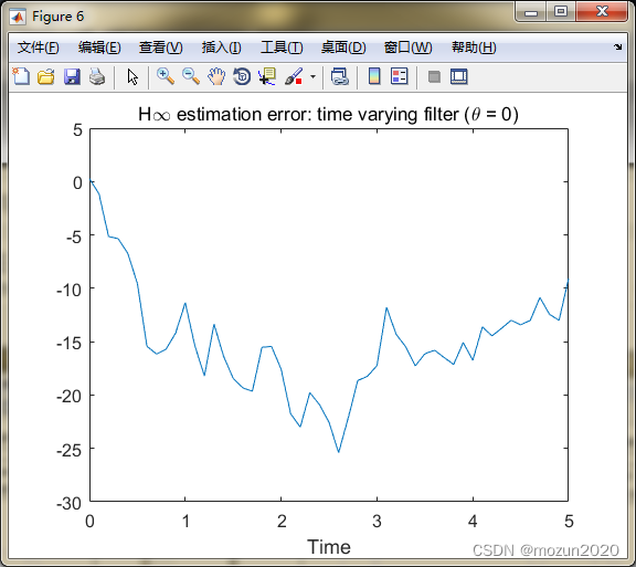
function HinfContEx1b
% Continuous time H-infinity filtering example
% INPUTS:
% theta = H-infinity performance bound
close all
[t, z0] = HinfFilter(0, 7/16);
[t, z1] = HinfFilter(1, 7/16);
[t, zk] = HinfFilter(0, 0);
figure;
plot(t,z0,'r-', t,z1,'b:');
set(gca,'FontSize',12); set(gcf,'Color','White');
xlabel('Time'); ylabel('Estimation Error');
legend('time varying filter', 'steady state filter');
figure;
plot(t,z0,'r-', t,zk,'b:');
set(gca,'FontSize',12); set(gcf,'Color','White');
xlabel('Time'); ylabel('Estimation Error');
legend('\theta = 7/16', '\theta = 0');
%%%%%%%%%%%%%%%%%%%%%%%%%%%%%%%%%%%%%%%%%%%%%%%%%%%%%%%%%%%%%%%%%%%
function [t, ztilde] = HinfFilter(SteadyState, theta)
% Initialize the random number generator seed.
% Try 0 and 1 for qualitatively different results.
randn('state', 0);
% Define system matrices.
A = 1;
C = 1;
L = 1;
Q = 1;
R = 1;
S = 1;
P = 1;
tf = 5; % simulation time
dt = 0.1; % simulation step size
x = 0; % initial state
xhat = 0; % initial state estimate
enorm = 0;
ztildenorm = 0;
% Create arrays for plotting data
zArray = [];
zhatArray = [];
for t = 0 : dt : tf
% Generate noise
w = 10 * randn(1);
v = 10 * randn(1);
v = 10 + v;
% Simulate system dynamics
xdot = A * x + w;
x = x + xdot * dt;
y = C * x + v;
z = L * x;
% Compute filter gain
if (SteadyState == 1)
K = 4;
else
K = P * C' * inv(R);
Pdot = A * P + P * A' + Q - K * C * P + theta * P * L' * S * L * P;
P = P + Pdot * dt;
end
% Filter dynamics
xhatdot = A * xhat + K * (y - C * xhat);
xhat = xhat + xhatdot * dt;
zhat = L * xhat;
% Save date for later plotting
zArray = [zArray z];
zhatArray = [zhatArray zhat];
% Compute integral of noise squared, and integral of estimation error
% squared.
enorm = enorm + (w^2 + v^2) * dt;
ztildenorm = ztildenorm + (z - zhat)^2 * dt;
end
% Plot data
t = 0 : dt : tf;
figure;
plot(t,zArray,'r', t,zhatArray,'b:');
if (SteadyState == 1)
TitleStr = 'H\infty filter simulation results: steady state filter';
else
TitleStr = 'H\infty filter simulation results: time varying filter';
end
title(TitleStr, 'FontSize', 12);
set(gca,'FontSize',12); set(gcf,'Color','White');
xlabel('Time'); ylabel('');
legend('true output', 'estimated output');
figure;
ztilde = zArray - zhatArray;
plot(t,ztilde);
if (SteadyState == 1)
TitleStr = 'H\infty estimation error: steady state filter (\theta = ';
else
TitleStr = 'H\infty estimation error: time varying filter (\theta = ';
end
TitleStr = [TitleStr, num2str(theta), ')'];
title(TitleStr, 'FontSize', 12);
set(gca,'FontSize',12); set(gcf,'Color','White');
xlabel('Time'); ylabel('');
disp(['infinity norm = ', num2str(sqrt(ztildenorm/enorm))]);

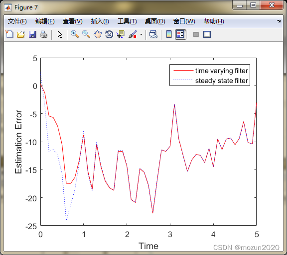
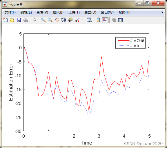
>> HinfContEx1b
infinity norm = 0.8206
infinity norm = 0.86263
infinity norm = 0.98192
5. 小结
运动控制在现代生活中的实际应用非常广泛,除了智能工厂中各种智能设备的自动运转控制,近几年最火的自动驾驶技术,以及航空航天领域,都缺少不了它的身影,所以熟练掌握状态估计理论,对未来就业也是非常有帮助的。切记矩阵理论与概率论等知识的基础一定要打好。对本章内容感兴趣或者想充分学习了解的,建议去研习书中第十一章节的内容,有条件的可以通过习题的联系进一步巩固充实。后期会对其中一些知识点在自己理解的基础上进行讨论补充,欢迎大家一起学习交流。
原书链接:Optimal State Estimation:Kalman, H-infinity, and Nonlinear Approaches


 801
801

 被折叠的 条评论
为什么被折叠?
被折叠的 条评论
为什么被折叠?
 到【灌水乐园】发言


