Topic 16. 临床预测模型之接收者操作特征曲线 (ROC)

最新推荐文章于 2024-01-13 15:45:12 发布

桓峰基因

最新推荐文章于 2024-01-13 15:45:12 发布

阅读量3.9k

点赞数 3

分类专栏：临床预测模型构建统计学分析方法文章标签：数据分析数据挖掘机器学习人工智能

本文链接：https://blog.csdn.net/weixin_41368414/article/details/124059493

版权

临床预测模型构建统计学分析方法专栏收录该内容

23 篇文章 124 订阅

订阅专栏

点击关注，桓峰基因

桓峰基因

生物信息分析，SCI文章撰写及生物信息基础知识学习：R语言学习，perl基础编程，linux系统命令，Python遇见更好的你

67篇原创内容

公众号

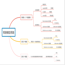
全网总结最全的 ROC 绘制方法，总有一款适合您！

前言

ROC（receiver operating characteristic curve）接收者操作特征曲线，是由二战中的电子工程师和雷达工程师发明用来侦测战场上敌军载具（飞机、船舰）的指标，属于信号检测理论。ROC曲线的横坐标是伪阳性率（也叫假正类率，False Positive Rate），纵坐标是真阳性率（真正类率，True Positive Rate），相应的还有真阴性率（真负类率，True Negative Rate）和伪阴性率（假负类率，False Negative Rate）。这四类指标的计算方法如下：

（1）伪阳性率（FPR）：判定为正例却不是真正例的概率，即真负例中判为正例的概率

（2）真阳性率（TPR）：判定为正例也是真正例的概率，即真正例中判为正例的概率（也即正例召回率）

（3）伪阴性率（FNR）：判定为负例却不是真负例的概率，即真正例中判为负例的概率。

（4）真阴性率（TNR）：判定为负例也是真负例的概率，即真负例中判为负例的概率。

原理

ROC（Receiver Operating Characteristic）曲线，又称接受者操作特征曲线。该曲线最早应用于雷达信号检测领域，用于区分信号与噪声。后来人们将其用于评价模型的预测能力，ROC曲线是基于混淆矩阵得出的。一个二分类模型的阈值可能设定为高或低，每种阈值的设定会得出不同的 FPR 和 TPR ，将同一模型每个阈值的 (FPR, TPR) 坐标都画在 ROC 空间里，就成为特定模型的ROC曲线。ROC曲线横坐标为假正率（FPR），纵坐标为真正率（TPR）。

主要作用

1.ROC曲线能很容易的查出任意阈值对学习器的泛化性能影响。

2.有助于选择最佳的阈值。ROC曲线越靠近左上角，模型的准确性就越高。最靠近左上角的ROC曲线上的点是分类错误最少的最好阈值，其假正例和假反例总数最少。

3.可以对不同的学习器比较性能。将各个学习器的ROC曲线绘制到同一坐标中，直观地鉴别优劣，靠近左上角的ROC曲所代表的学习器准确性最高。

优点

该方法简单、直观、通过图示可观察分析学习器的准确性，并可用肉眼作出判断。ROC曲线将真正例率和假正例率以图示方法结合在一起，可准确反映某种学习器真正例率和假正例率的关系，是检测准确性的综合代表。ROC曲线不固定阈值，允许中间状态的存在，利于使用者结合专业知识，权衡漏诊与误诊的影响，选择一个更加的阈值作为诊断参考值。AUC（Area Under Curve）被定义为ROC曲线下的面积。我们往往使用AUC值作为模型的评价标准是因为很多时候ROC曲线并不能清晰的说明哪个分类器的效果更好，而作为一个数值，对应AUC更大的分类器效果更好。其中，ROC曲线全称为受试者工作特征曲线（receiver operating characteristic curve），它是根据一系列不同的二分类方式（分界值或决定阈），以真阳性率（敏感性）为纵坐标，假阳性率（1-特异性）为横坐标绘制的曲线。

AUC就是衡量学习器优劣的一种性能指标。从定义可知，AUC可通过对ROC曲线下各部分的面积求和而得. AUC就是曲线下面积，在比较不同的分类模型时，可以将每个模型的ROC曲线都画出来，比较曲线下面积做为模型优劣的指标。ROC 曲线下方的面积(Area under the Curve)，其意义是：（1）因为是在1x1的方格里求面积，AUC必在0~1之间。

（2）假设阈值以上是阳性，以下是阴性；

（3）若随机抽取一个阳性样本和一个阴性样本，分类器正确判断阳性样本的值高于阴性样本的概率 = AUC 。

（4）简单说：AUC值越大的分类器，正确率越高。

从AUC 判断分类器（预测模型）优劣的标准：

AUC = 1，是完美分类器。

AUC = [0.85, 0.95], 效果很好

AUC = [0.7, 0.85], 效果一般

AUC = [0.5, 0.7],效果较低，但用于预测股票已经很不错了

AUC = 0.5，跟随机猜测一样（例：丢铜板），模型没有预测价值。

AUC < 0.5，比随机猜测还差；但只要总是反预测而行，就优于随机猜测。

如果两条ROC曲线没有相交，我们可以根据哪条曲线最靠近左上角哪条曲线代表的学习器性能就最好。但是，实际任务中，情况很复杂，如果两条ROC曲线发生了交叉，则很难一般性地断言谁优谁劣。在很多实际应用中，我们往往希望把学习器性能分出个高低来。在此引入AUC面积。在进行学习器的比较时，若一个学习器的ROC曲线被另一个学习器的曲线完全“包住”，则可断言后者的性能优于前者；若两个学习器的ROC曲线发生交叉，则难以一般性的断言两者孰优孰劣。此时如果一定要进行比较，则比较合理的判断依据是比较ROC曲线下的面积，即AUC(Area Under ROC Curve)。

实例解析

这期我们总结了几种实现方法，方便大家选择性使用，但是最终目的是一样，实现最后的结果也是一致的。

1. 软件安装并加载

这里介绍几个R软件包的实现方法，安装并加载这些软件包，如下：

if (!require(survivalROC)) {
    install.packages("survivalROC")
}
if (!require(pROC)) {
    install.packages("pROC")
}
if (!require(ROCR)) {
    install.packages("ROCR")
}
## Warning: 程辑包'ROCR'是用R版本4.1.3 来建造的
if (!require(AUC)) {
    install.packages("AUC")
}
## Warning: 程辑包'AUC'是用R版本4.1.3 来建造的
if (!require(timeROC)) {
    install.packages("timeROC")
}
## Warning: 程辑包'timeROC'是用R版本4.1.3 来建造的
if (!require(plotROC)) {
    install.packages("plotROC")
}
## Warning: 程辑包'plotROC'是用R版本4.1.3 来建造的

library(survivalROC)
library(pROC)
library(ROCR)
library(AUC)
library(timeROC)
library(plotROC)
library(survival)

2. 数据读取

我们选择Mayo PBC 数据集带有生存信息，在 survivalROC 软件包中，如下：

Format A data frame with 312 observations and 4 variables: time (event time/censoring time), censor (censoring indicator), mayoscore4, mayoscore5. The two scores are derived from 4 and 5 covariates respectively.

读取数据，如下：

library(survivalROC)
data(mayo)
str(mayo)
## 'data.frame':	312 obs. of  4 variables:
##  $ time      : int  41 179 334 400 130 223 51 549 216 859 ...
##  $ censor    : int  1 1 1 1 1 1 1 1 1 1 ...
##  $ mayoscore5: num  11.25 10.14 10.1 10.19 9.77 ...
##  $ mayoscore4: num  10.63 10.19 9.42 9.57 9.04 ...
head(mayo)
##   time censor mayoscore5 mayoscore4
## 1   41      1  11.251850  10.629450
## 2  179      1  10.136070  10.185220
## 3  334      1  10.095740   9.422995
## 4  400      1  10.189150   9.567799
## 5  130      1   9.770148   9.039419
## 6  223      1   9.226429   9.033388

3. 绘制AUC曲线

这里我们选择五种方式绘制AUC曲线，每种方式略有不同，但是其结果应该是一致的。

1.survivalROC{survivalROC}

SurvivalROC包绘制时间依赖的ROC曲线.假设我们有删失的生存数据与基线marker值，我们希望看到marker如何预测数据集中的受试者的存活时间。特别是，假设我们有几天的生存时间，我们想看看标记如何预测一年的存活（predict.time=365）。该功能roc.km.calc()返回感兴趣的时间点的唯一标记值、TP（真阳性）、FP（假阳性）、对应于感兴趣时间点(predict.time)和AUC(ROC)曲线下面积的Kaplan-Meier生存估计。survivalROC返回值说明如下：

cut.values:由于计算TP和FP的marker值
TP: 根据cutoff 判断的TRUE postive 真阳性
FP: 根据cutoff判断的假阳性
predict.time: 感兴趣的时间截点：可以为5年，3年等等
Survival: kaplan-Meier法的预估生存时间
AUC: Area under ROC，在时间截点的曲线下面积

根据返回值我们可以计算cutoff阈值，ROC的最佳阈值（cutoff）一般来说，对于一个biomarker或者简单的说诊断指标/试剂，我们使用ROC曲线计算出AUC值后，还会根据ROC曲线的最佳阈值来确定其灵敏度和特异度，有时在研究中，还会用于KM曲线的分类指标确定阈值的方法很多（可参考：ROC Curve或者One ROC Curve and Cutoff Analysis），一般会用最常见的约登指数(Youden index)，即敏感度+特异性-1；有时也会考虑用其他确定阈值的方法，比如Minimum ROC distance, Misclassification Cost Term等等（参考：ROC）

对于上述timeROC的结果，如3年ROC曲线的约登指数（因为TP代表的是True Positive fraction，即sensitivity；而FP代表的是False Positive fraction，即1-specificity）,通过换算之后即为即sensitivity-specificity取最大值的那个mayoscore4作为最佳阈值（cutoff）为5.756277

library(RColorBrewer)
rocCol=brewer.pal(8,"Set1")
aucText=c()

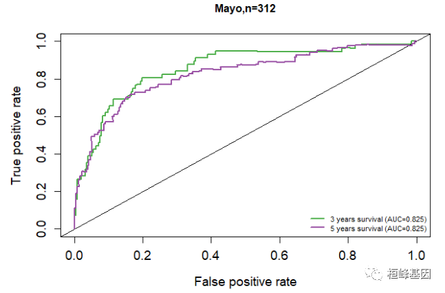
roc=survivalROC(Stime=mayo$time, ##生存时间
                status=mayo$censor, ## 终止事件
                marker = mayo$mayoscore4, ## risk score
                predict.time =1068, ## 预测时间截点
                method="KM")
#span = 0.25*nobs^(-0.20))##span,NNE法的namda)
roc$AUC
## [1] 0.8561212

plot(roc$FP, roc$TP, type="l", xlim=c(0,1), ylim=c(0,1),col=rocCol[3], 
     xlab="False positive rate", ylab="True positive rate",
     lwd = 2, cex.main=1, cex.lab=1.2, cex.axis=1.2, font=1.2,
     main=paste0("Mayo,n=",nrow(mayo)))

roc=survivalROC(Stime=mayo$time, status=mayo$censor, marker = mayo$mayoscore4, 
                predict.time =1780, method="KM")
aucText=c(aucText,paste0("3 years survival"," (AUC=",sprintf("%.3f",roc$AUC),")"))
abline(0,1)
aucText=c(aucText,paste0("5 years survival"," (AUC=",sprintf("%.3f",roc$AUC),")"))
lines(roc$FP, roc$TP, type="l", xlim=c(0,1), ylim=c(0,1),col=rocCol[4],lwd = 2)
legend("bottomright", aucText,lwd=2,bty="n",col=rocCol[c(3,4)],cex = 0.7)

对于上述survivalROC的结果，如5年ROC曲线的约登指数（因为TP代表的是True Positive fraction，即sensitivity；而FP代表的是False Positive fraction，即1-specificity）,通过换算之后即为即sensitivity-specificity取最大值的那个mayoscore4作为最佳阈值（cutoff）为6.834187

roc_res <- data.frame(roc$TP, roc$FP)
colnames(roc_res) = c("TP", "FP")
roc_res[which.max(roc_res$TP - roc_res$FP) - 1, ]
##           TP        FP
## 212 0.716723 0.1671751
mayo$mayoscore4[212]
## [1] 6.834187

2.auc{pROC}

pROC是一个相对plotROC更强大的R包，不同于plotROC基于ggplot2的创建，pROC自身构建了比较完整的ROC分析和绘图体系。不过相对于plotROC，它的图形绘制更为复杂,如下：

plot.roc(mayo$censor, mayo$mayoscore4, # data
         percent=TRUE, # show all values in percent
         partial.auc=c(100, 90), 
         partial.auc.correct=TRUE, # define a partial AUC (pAUC)
         print.auc=TRUE, #display pAUC value on the plot with following options:
         print.auc.pattern="pAUC of mayoscore4: %.1f%%", print.auc.col="#1c61b6",
         auc.polygon=TRUE, 
         auc.polygon.col="#1c61b6", # show pAUC as a polygon
         max.auc.polygon=TRUE, 
         max.auc.polygon.col="#1c61b622", # also show the 100% polygon
         main="Partial AUC (pAUC)"
         )

plot.roc(mayo$censor, mayo$mayoscore5,
         percent=TRUE, add=TRUE, type="n", # add to plot, but don't re-add the ROC itself (useless)
         partial.auc=c(100, 90), partial.auc.correct=TRUE,
         partial.auc.focus="se", # focus pAUC on the sensitivity
         print.auc=TRUE, 
         print.auc.pattern="pAUC of mayoscore5: %.1f%%", 
         print.auc.col="#008600",
         print.auc.y=40, # do not print auc over the previous one
         auc.polygon=TRUE, auc.polygon.col="#008600",
         max.auc.polygon=TRUE, max.auc.polygon.col="#00860022")

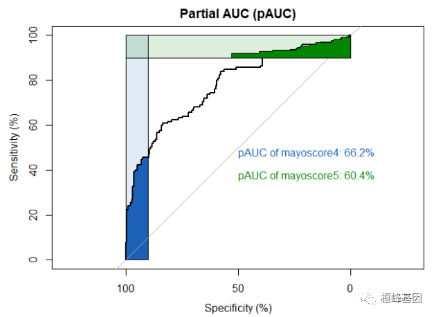
这样的图形，我们参考代码修改和自定义即可。这个图显示了pROC包最重要几个函数的使用，第一个是plot.roc()，它可以绘制ROC曲线，并返回一个ROC对象，里面包含该曲线的众多有用信息，并为后续的分析做基础，lines.roc()为当前ROC曲线上增添新的ROC曲线。不仅如此，roc.test()函数提供了对曲线进行检验，检验的方法分为3种，可以自己选择，有兴趣的朋友不妨再深入看看

rocobj1 <- plot.roc(mayo$censor, mayo$mayoscore4, main = "Statistical comparison",
    percent = TRUE, col = "#1c61b6", xlim = c(100, 0), ylim = c(0, 100))
rocobj1
## 
## Call:
## plot.roc.default(x = mayo$censor, predictor = mayo$mayoscore4,     main = "Statistical comparison", percent = TRUE, col = "#1c61b6",     xlim = c(100, 0), ylim = c(0, 100))
## 
## Data: mayo$mayoscore4 in 187 controls (mayo$censor 0) < 125 cases (mayo$censor 1).
## Area under the curve: 77.51%
rocobj2 <- lines.roc(mayo$censor, mayo$mayoscore5, percent = TRUE, col = "#008600")
rocobj2
## 
## Call:
## lines.roc.default(x = mayo$censor, predictor = mayo$mayoscore5,     percent = TRUE, col = "#008600")
## 
## Data: mayo$mayoscore5 in 187 controls (mayo$censor 0) < 125 cases (mayo$censor 1).
## Area under the curve: 84.56%
testobj <- roc.test(rocobj1, rocobj2)
testobj
## 
## 	DeLong's test for two correlated ROC curves
## 
## data:  rocobj1 and rocobj2
## Z = -3.5896, p-value = 0.0003312
## alternative hypothesis: true difference in AUC is not equal to 0
## 95 percent confidence interval:
##  -0.10893175 -0.03198804
## sample estimates:
## AUC of roc1 AUC of roc2 
##    77.51444    84.56043
auc = round(c(testobj$roc1$auc[1], testobj$roc2$auc[1]), 1)
auc = paste(auc, "%", sep = "")
text(50, 50, labels = paste("p-value =", format.pval(testobj$p.value)), adj = c(0,
    0.5))
legend("bottomright", legend = paste(c("mayoscore4", "mayoscore5"), auc, sep = ": "),
    col = c("#1c61b6", "#008600"), lwd = 2, bty = "n")

3. performance{ROCR}

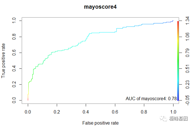
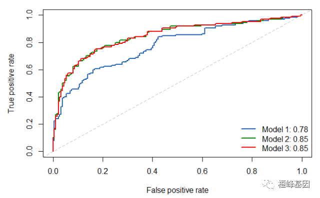
我们仍然使用mayo数据集，构建Logistic回归模型，获得预测值，在计算AUC，并绘制单个变量与联合变量预测模型的比较，我们发现mayoscore5 与联合两个变量的AUC结果一致，故该变量的预测结果最好，如下：

Model1 <- glm(censor ~ mayoscore4, data = mayo)
Model2 <- glm(censor ~ mayoscore5, data = mayo)
Model3 <- glm(censor ~ mayoscore4 + mayoscore5, data = mayo)
### Model 1
mayo$predvalue1 <- predict(Model1, type = "response")
pred1 <- prediction(mayo$predvalue1, mayo$censor)
perf1 <- performance(pred1, "tpr", "fpr")
# 计算AUC，结果返回一个S4对象，y.values就是AUC
auc1 <- performance(pred1, "auc")
## S4对象，其内包括6个数据##
slotNames(auc1)
## [1] "x.name"       "y.name"       "alpha.name"   "x.values"     "y.values"    
## [6] "alpha.values"
# AUC数值如下

auc[1] <- auc1@y.values[[1]]
auc[1] = round(as.numeric(auc[1]), 2)
####### Model 2
mayo$predvalue2 <- predict(Model2, type = "response")
pred2 <- prediction(mayo$predvalue2, mayo$censor)
perf2 <- performance(pred2, "tpr", "fpr")
# 计算AUC，结果返回一个S4对象，y.values就是AUC
auc2 <- performance(pred2, "auc")
## S4对象，其内包括6个数据##
slotNames(auc2)
## [1] "x.name"       "y.name"       "alpha.name"   "x.values"     "y.values"    
## [6] "alpha.values"
# AUC数值如下
auc[2] <- auc2@y.values[[1]]
auc[2] = round(as.numeric(auc[2]), 2)
##### Model 3
mayo$predvalue3 <- predict(Model3, type = "response")
pred3 <- prediction(mayo$predvalue3, mayo$censor)
perf3 <- performance(pred3, "tpr", "fpr")
# 计算AUC，结果返回一个S4对象，y.values就是AUC
auc3 <- performance(pred3, "auc")
## S4对象，其内包括6个数据##
slotNames(auc3)
## [1] "x.name"       "y.name"       "alpha.name"   "x.values"     "y.values"    
## [6] "alpha.values"
# AUC数值如下
auc[3] <- auc3@y.values[[1]]
auc[3] = round(as.numeric(auc[3]), 2)
auc
## [1] "0.78" "0.85" "0.85"

单个AUC曲线绘制，如下：

plot(perf1, colorize = TRUE, main = "mayoscore4", box.lty = 7, box.lwd = 2, box.col = "gray")
legend("bottomright", legend = paste("AUC of mayoscore4", auc[1], sep = ": "), col = "#1c61b6",
    bty = "n")

多个AUC曲线在一张图上，如下：

######### 作图
plot(perf1, col = "#1c61b6", lwd = 2)
plot(perf2, col = "#008600", lwd = 2, add = T)
plot(perf3, col = "red", lwd = 2, add = T)
abline(0, 1, lty = 2, col = "gray")
legend("bottomright", legend = paste(c("Model 1", "Model 2", "Model 3"), auc, sep = ": "),
    col = c("#1c61b6", "#008600", "red"), lwd = 2, bty = "n")

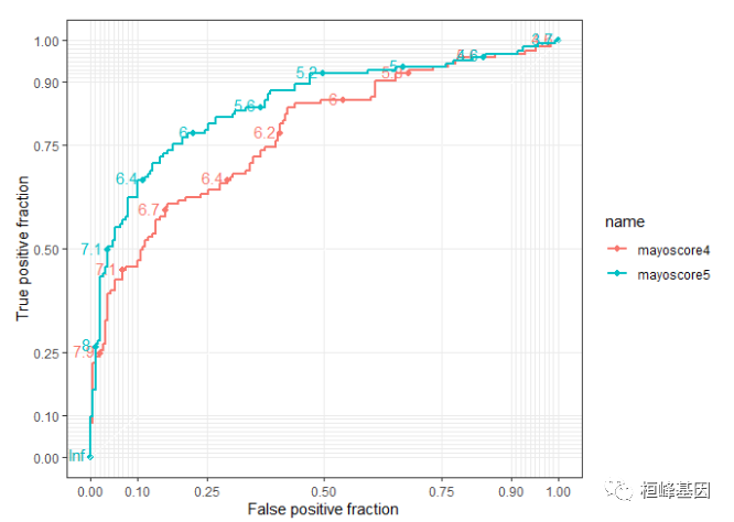
4. geom_roc{plotROC}

plotROC包较为简单与单一，它就是用来绘制ROC曲线的，包中定义的函数基于ggplot2，因此我们可以结合ggplot2使用和修改、美化图形结果。默认曲线上会显示阈值cutoff的数值。

library(ggplot2)
set.seed(1234)
basicplot <- ggplot(mayo, aes(d = censor, m = mayoscore4)) + geom_roc()
basicplot

plotROC提供的函数melt_roc()可以将多个变量列变为长格式，方便数据的绘制：

longtest <- melt_roc(mayo, "censor", c("mayoscore4", "mayoscore5"))
head(longtest)
##             D         M       name
## mayoscore41 1 10.629450 mayoscore4
## mayoscore42 1 10.185220 mayoscore4
## mayoscore43 1  9.422995 mayoscore4
## mayoscore44 1  9.567799 mayoscore4
## mayoscore45 1  9.039419 mayoscore4
## mayoscore46 1  9.033388 mayoscore4
ggplot(longtest, aes(d = D, m = M, color = name)) + geom_roc() + style_roc()

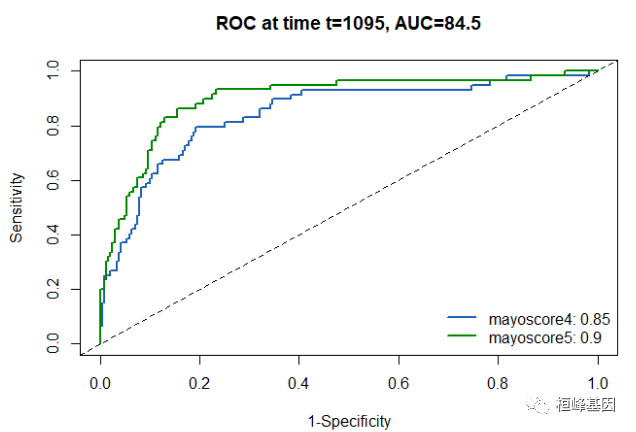
5. timeROC{timeROC}

timeROC估计多个时间点AUC以及AUC的95%置信区间。使用timeROC绘制mayoscore5与mayoscore4在不同时间点的ROC曲线，以及不同时间点的AUC。

# evaluate mayoscore4-5 as a prognostic biomarker
mayoscore4 <- timeROC(T = mayo$time, delta = mayo$censor, marker = mayo$mayoscore4,
    cause = 1, weighting = "marginal", times = c(365 * 1, 365 * 2, 365 * 3, 365 *
        4, 365 * 5, 365 * 6, 365 * 7, 365 * 8, 365 * 9, 365 * 10), ROC = TRUE, iid = TRUE)
mayoscore5 <- timeROC(T = mayo$time, delta = mayo$censor, marker = mayo$mayoscore5,
    cause = 1, weighting = "marginal", times = c(365 * 1, 365 * 2, 365 * 3, 365 *
        4, 365 * 5, 365 * 6, 365 * 7, 365 * 8, 365 * 9, 365 * 10), ROC = TRUE, iid = TRUE)
# computes pointwise confidence interval
ci_4 <- confint(mayoscore4)
ci_4
## $CI_AUC
##         2.5%  97.5%
## t=365  83.22 100.26
## t=730  81.47  96.70
## t=1095 78.61  90.48
## t=1460 77.49  89.52
## t=1825 77.14  88.57
## t=2190 73.04  85.80
## t=2555 72.18  85.04
## t=2920 64.68  80.38
## t=3285 65.89  82.15
## t=3650 68.17  85.19
## 
## $CB_AUC
##         2.5%  97.5%
## t=365  80.18 103.30
## t=730  78.75  99.43
## t=1095 76.49  92.60
## t=1460 75.34  91.68
## t=1825 75.10  90.61
## t=2190 70.76  88.08
## t=2555 69.88  87.34
## t=2920 61.87  83.18
## t=3285 62.98  85.06
## t=3650 65.13  88.23
## 
## $C.alpha
##      95% 
## 2.660692
ci_5 <- confint(mayoscore5)
ci_5
## $CI_AUC
##         2.5%  97.5%
## t=365  83.56 100.05
## t=730  79.28  95.37
## t=1095 85.01  94.64
## t=1460 86.94  95.79
## t=1825 87.42  95.65
## t=2190 82.99  93.55
## t=2555 80.66  92.15
## t=2920 74.29  87.89
## t=3285 75.33  88.86
## t=3650 79.38  92.14
## 
## $CB_AUC
##         2.5%  97.5%
## t=365  80.69 102.92
## t=730  76.48  98.17
## t=1095 83.34  96.32
## t=1460 85.40  97.32
## t=1825 85.99  97.08
## t=2190 81.16  95.39
## t=2555 78.66  94.15
## t=2920 71.93  90.25
## t=3285 72.98  91.21
## t=3650 77.17  94.36
## 
## $C.alpha
##     95% 
## 2.64128
auc_res = round(c(mayoscore4$AUC[3], mayoscore5$AUC[3]), 2)
# Plot the RoC curveat time t=365*1
plot(mayoscore4, time = 365 * 3, col = "#1c61b6", lwd = 2)
plot(mayoscore5, time = 365 * 3, col = "#008600", lwd = 2, add = T)
legend("bottomright", legend = paste(c("mayoscore4", "mayoscore5"), auc_res, sep = ": "),
    col = c("#1c61b6", "#008600"), lwd = 2, bty = "n")

绘制AUC曲线带有时间点的CI 置信区间，如下：

# plot AuC curve for mayoscore4 only with pointwise CI
plotAUCcurve(mayoscore4, FP = 2, add = FALSE, conf.int = TRUE, conf.band = FALSE,
    col = "#1c61b6")

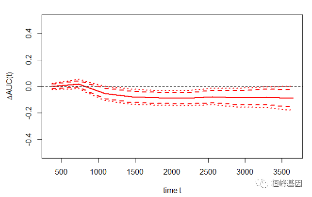
这个函数绘制了两个随时间变化的AUCs的差随时间的曲线。当用Kaplan-Meier估计器计算截尾权的逆概率时，也可以绘制该曲线的点区和置信区。

plotAUCcurveDiff(mayoscore4, mayoscore5, FP = 2, conf.int = TRUE, conf.band = TRUE,
    col = "red")

关注桓峰基因，每天更新不停息，有需要作图，SCI文章合作等，都可以找桓峰基因解决！

References:

Chambers, J. M. and Hastie, T. J. (1992) Statistical Models in S. Wadsworth & Brooks/Cole.
Heagerty, P.J., Zheng, Y. (2005) Survival Model Predictive Accuracy and ROC Curves Biometrics, 61, 92 – 105.
Xavier Robin, Natacha Turck, Alexandre Hainard, et al. (2011) “pROC: an open-source package for R and S+ to analyze and compare ROC curves”. BMC Bioinformatics, 7, 77.
Ballings, M., Van den Poel, D., Threshold Independent Performance Measures for Probabilistic Classifcation Algorithms, Forthcoming. Hung, H. and Chiang, C. (2010). Estimation methods for time-dependent AUC with survival data. Canadian Journal of Statistics, 38(1):8-26
Uno, H., Cai, T., Tian, L. and Wei, L. (2007). Evaluating prediction rules for t-years survivors with censored regression models. Journal of the American Statistical Association, 102(478):527-537.
Blanche, P., Dartigues, J. F., & Jacqmin-Gadda, H. (2013). Estimating and comparing time-dependent areas under receiver operating characteristic curves for censored event times with competing risks. Statistics in medicine, 32(30), 5381-5397.
P. Blanche, A. Latouche, V. Viallon (2013). Time-dependent AUC with right-censored data: A Survey. Risk Assessment and Evaluation of Predictions, 239-251, Springer,