


简 介
失效时间数据
根据生存结局的发生情况,生存分析的数据资料常常分为终点事件(如死亡)和删失(其他生存结局)两类。
生存分析不同类型的数据包括:
完全数据(Complete data)
删失数据(Censoring data)
删失数据通常在其右上角标记"+"号,表示真实的生存时间未知,只知道比观察到的删失时间要长。在生存分析中,发生终点事件记为“1” ,删失记为"0” 。
删失的类型包括:
(1) 右删失(Right censored)
I型删失(Type I censoring)
II型删失(Type II censoring)
III型删失(Type II censoring)
(注:图中X表示发生终点事件,O示删失)
(2) 左删失(Left censored)
(3) 区间删失(Interval censored)
生存分析方法分类
1. 参数法--survreg()
假定生存时间服从某个特定的分布,然后根据分布的特点对生存时间进行分析,常用方法有指数分布法、weibull分步法、对数正态回归分布法等。参数法通过估计的参数得到生存率的估计值,对于两组及多组的样本可根据参数估计对其进行统计推断。早期应用于武器使用寿命的研究等。
2. 半参数法--coxph()
只规定了影响因素和生存状况间的关系,但是没对时间(和风险函数)的分布情况加以限定。这种方法主要用于分析生存率的影响因素,属于多因素分析方法,典型方法是cox比例风险模型。Cox模型分析法以风险率函数作为应变量,以与生存时间可能有关的协变量或交互项作为自变量来分析生存率。
3. 非参数法--survdiff()
根据样本的顺序统计量对生存率进行估计,常用的方法有log-rank检验、似然比检验,对于两个及多个生存率的比较,其零假设为两组或多组总体生存时间分布相同,而不对其具体的分布形式及参数进行推断。常用于随访资料医学研究。
缺失类型-Surv()
缺失类型选择可以通过surv()函数中的type参数来选择:
type=c('right', 'left', 'interval', 'counting', 'interval2', 'mstate'),
character string specifying the type of censoring. Possible values are "right", "left", "counting", "interval", "interval2" or "mstate".
今天介绍的是拟合参数生存回归模型的构建--survreg()。
软件包安装
if(require(survival))
  install.packages("survival")
数据读取
数据说明:
futime: survival or censoring time
fustat: censoring status
age: in years
resid.ds: residual disease present (1=no,2=yes)
rx: treatment group
ecog.ps: ECOG performance status (1 is better, see reference)
data(cancer, package="survival")
head(ovarian)
## futime fustat age resid.ds rx ecog.ps
## 1 59 1 72.3315 2 1 1
## 2 115 1 74.4932 2 1 1
## 3 156 1 66.4658 2 1 2
## 4 421 0 53.3644 2 2 1
## 5 431 1 50.3397 2 1 1
## 6 448 0 56.4301 1 1 2实例操作
参数说明:
survreg(formula, data, weights, subset,
        na.action, dist="weibull", init=NULL, scale=0,
        control,parms=NULL,model=FALSE, x=FALSE,
        y=TRUE, robust=FALSE, cluster, score=FALSE, ...)

formula
a formula expression as for other regression models. The response is usually a survival object as returned by the Surv function. See the documentation for Surv, lm and formula for details.

data
a data frame in which to interpret the variables named in the formula, weights or the subset arguments.

weights
optional vector of case weights

subset
subset of the observations to be used in the fit

na.action
a missing-data filter function, applied to the model.frame, after any subset argument has been used. Default is options()\$na.action.

dist
assumed distribution for y variable. If the argument is a character string, then it is assumed to name an element from survreg.distributions. These include "weibull", "exponential", "gaussian", "logistic","lognormal" and "loglogistic". Otherwise, it is assumed to be a user defined list conforming to the format described in survreg.distributions.

parms
a list of fixed parameters. For the t-distribution for instance this is the degrees of freedom; most of the distributions have no parameters.

init
optional vector of initial values for the parameters.

scale
optional fixed value for the scale. If set to <=0 then the scale is estimated.

control
a list of control values, in the format produced by survreg.control. The default value is survreg.control()

model, x, y
flags to control what is returned. If any of these is true, then the model frame, the model matrix, and/or the vector of response times will be returned as components of the final result, with the same names as the flag arguments.

score
return the score vector. (This is expected to be zero upon successful convergence.)

robust
Use robust sandwich error instead of the asymptotic formula. Defaults to TRUE if there is a cluster argument.

cluster
Optional variable that identifies groups of subjects, used in computing the robust variance. Like model variables, this is searched for in the dataset pointed to by the data argument.

...
other arguments which will be passed to survreg.control.
构建模型
根据说明ovarian数据集,构建模型:
library(survival)
fit <- survreg(Surv(futime, fustat) ~ ., ovarian, dist = "weibull", scale = 1)
summary(fit)
##
## Call:
## survreg(formula = Surv(futime, fustat) ~ ., data = ovarian, dist = "weibull",
##     scale = 1)
##               Value Std. Error     z       p
## (Intercept) 12.7826     2.5137  5.09 3.7e-07
## age         -0.0875     0.0338 -2.59  0.0096
## resid.ds    -0.7659     0.7411 -1.03  0.3014
## rx           0.6269     0.6162  1.02  0.3090
## ecog.ps     -0.2523     0.6061 -0.42  0.6772
##
## Scale fixed at 1
##
## Weibull distribution
## Loglik(model)= -90.6   Loglik(intercept only)= -98
## 	Chisq= 14.78 on 4 degrees of freedom, p= 0.0052
## Number of Newton-Raphson Iterations: 5
## n= 26
筛选最优模型
若要找到最佳模型,可以进行变量选择,采用逐步回归法进行分析,最后找到age显著。
library(MASS)
stepVar <- stepAIC(fit, direction = "both")
## Start:  AIC=191.29
## Surv(futime, fustat) ~ age + resid.ds + rx + ecog.ps
##
##            Df    AIC
## - ecog.ps   1 189.46
## - rx        1 190.31
## - resid.ds  1 190.39
## <none>        191.29
## - age       1 198.05
##
## Step:  AIC=189.46
## Surv(futime, fustat) ~ age + resid.ds + rx
##
##            Df    AIC
## - resid.ds  1 188.42
## - rx        1 188.44
## <none>        189.46
## + ecog.ps   1 191.29
## - age       1 196.73
##
## Step:  AIC=188.42
## Surv(futime, fustat) ~ age + rx
##
##            Df    AIC
## - rx        1 187.56
## <none>        188.42
## + resid.ds  1 189.46
## + ecog.ps   1 190.39
## - age       1 198.95
##
## Step:  AIC=187.56
## Surv(futime, fustat) ~ age
##
##            Df    AIC
## <none>        187.56
## + rx        1 188.42
## + resid.ds  1 188.44
## + ecog.ps   1 189.55
## - age       1 198.06
summary(stepVar)
##
## Call:
## survreg(formula = Surv(futime, fustat) ~ age, data = ovarian,
## dist = "weibull", scale = 1)
## Value Std. Error z p
## (Intercept) 13.9339 2.1030 6.63 3.5e-11
## age -0.1185 0.0339 -3.50 0.00047
##
## Scale fixed at 1
##
## Weibull distribution
## Loglik(model)= -91.8 Loglik(intercept only)= -98
## Chisq= 12.51 on 1 degrees of freedom, p= 0.00041
## Number of Newton-Raphson Iterations: 5
## n= 26optFit <- survreg(Surv(futime, fustat) ~ age, ovarian, dist = "weibull", scale = 1)一致性
C_index <- data.frame(Cindex = as.numeric(summary(coxph(Surv(futime, fustat) ~ age,
    data = ovarian))$concordance[1]))
C_index
##      Cindex
## 1 0.7844037
生存分析
根据最优解,模型中只有age这个变量,所以直接做生存分析即可:
library(survminer)
ovarian$age = ifelse(ovarian$age > median(ovarian$age), "High", "Low")
f <- survfit(Surv(futime, fustat) ~ age, data = ovarian)
ggsurvplot(f, data = ovarian, surv.median.line = "hv", legend.title = "Risk Group",
    legend.labs = c("High Risk", "Low Risk"), pval = TRUE, ggtheme = theme_bw())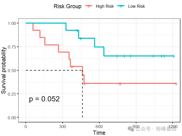
验证
ovarian$resposnse <- predict(optFit, newdata = ovarian, type = "response")绘制ROC曲线
library(pROC)
roc <- roc(ovarian$fustat, ovarian$resposnse, legacy.axes = T, print.auc = T, print.auc.y = 45)
roc$auc
## Area under the curve: 0.6548
plot(roc, legacy.axes = T, col = "red", lwd = 2, main = "ROC curv")
text(0.2, 0.2, paste("AUC: ", round(roc$auc, 2)))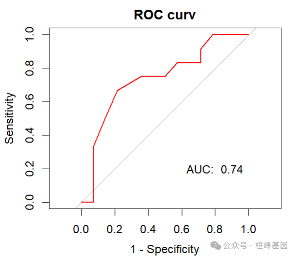
Reference
Kalbfleisch, J. D. and Prentice, R. L., The statistical analysis of failure time data, Wiley, 2002.
基于机器学习构建临床预测模型
MachineLearning 2. 因子分析(Factor Analysis)
MachineLearning 3. 聚类分析(Cluster Analysis)
MachineLearning 4. 癌症诊断方法之 K-邻近算法(KNN)
MachineLearning 5. 癌症诊断和分子分型方法之支持向量机(SVM)
MachineLearning 6. 癌症诊断机器学习之分类树(Classification Trees)
MachineLearning 7. 癌症诊断机器学习之回归树(Regression Trees)
MachineLearning 8. 癌症诊断机器学习之随机森林(Random Forest)
MachineLearning 9. 癌症诊断机器学习之梯度提升算法(Gradient Boosting)
MachineLearning 10. 癌症诊断机器学习之神经网络(Neural network)
MachineLearning 11. 机器学习之随机森林生存分析(randomForestSRC)
MachineLearning 12. 机器学习之降维方法t-SNE及可视化(Rtsne)
MachineLearning 13. 机器学习之降维方法UMAP及可视化 (umap)
MachineLearning 14. 机器学习之集成分类器(AdaBoost)
MachineLearning 15. 机器学习之集成分类器(LogitBoost)
MachineLearning 16. 机器学习之梯度提升机(GBM)
MachineLearning 17. 机器学习之围绕中心点划分算法(PAM)
MachineLearning 18. 机器学习之贝叶斯分析类器(Naive Bayes)
MachineLearning 19. 机器学习之神经网络分类器(NNET)
MachineLearning 20. 机器学习之袋装分类回归树(Bagged CART)
MachineLearning 21. 机器学习之临床医学上的生存分析(xgboost)
MachineLearning 22. 机器学习之有监督主成分分析筛选基因(SuperPC)
MachineLearning 23. 机器学习之岭回归预测基因型和表型(Ridge)
MachineLearning 24. 机器学习之似然增强Cox比例风险模型筛选变量及预后估计(CoxBoost)
MachineLearning 25. 机器学习之支持向量机应用于生存分析(survivalsvm)
MachineLearning 26. 机器学习之弹性网络算法应用于生存分析(Enet)
MachineLearning 27. 机器学习之逐步Cox回归筛选变量(StepCox)
MachineLearning 28. 机器学习之偏最小二乘回归应用于生存分析(plsRcox)
MachineLearning 29. 机器学习之嵌套交叉验证(Nested CV)
MachineLearning 30. 机器学习之特征选择森林之神(Boruta)
MachineLearning 31. 机器学习之基于RNA-seq的基因特征筛选 (GeneSelectR)
MachineLearning 32. 机器学习之支持向量机递归特征消除的特征筛选 (mSVM-RFE)
MachineLearning 33. 机器学习之时间-事件预测与神经网络和Cox回归
MachineLearning 34. 机器学习之竞争风险生存分析的深度学习方法(DeepHit)
MachineLearning 35. 机器学习之Lasso+Cox回归筛选变量 (LassoCox)
MachineLearning 36. 机器学习之基于神经网络的Cox比例风险模型 (Deepsurv)
MachineLearning 37. 机器学习之倾斜随机生存森林 (obliqueRSF)
MachineLearning 38. 机器学习之基于最近收缩质心分类法的肿瘤亚型分类器 (pamr)
MachineLearning 39. 机器学习之基于条件随机森林的生存分析临床预测 (CForest)
桓峰基因,铸造成功的您!
未来桓峰基因公众号将不间断的推出机器学习系列生信分析教程,
敬请期待!!
桓峰基因官网正式上线,请大家多多关注,还有很多不足之处,大家多多指正!http://www.kyohogene.com/
桓峰基因和投必得合作,文章润色优惠85折,需要文章润色的老师可以直接到网站输入领取桓峰基因专属优惠券码:KYOHOGENE,然后上传,付款时选择桓峰基因优惠券即可享受85折优惠哦!https://www.topeditsci.com/


 被折叠的 条评论
为什么被折叠?
被折叠的 条评论
为什么被折叠?
 到【灌水乐园】发言


