PatchCore代码详解 | Towards Total Recall in Industrial Anomaly Detection

洋芋焖土豆

已于 2024-06-17 16:46:15 修改

阅读量662

点赞数 20

分类专栏：缺陷检测文章标签：目标检测论文笔记

于 2024-06-17 11:01:27 首次发布

本文链接：https://blog.csdn.net/weixin_42355902/article/details/139738281

版权

缺陷检测专栏收录该内容

5 篇文章 0 订阅

订阅专栏

文章目录

Towards Total Recall in Industrial Anomaly Detection

Towards Total Recall in Industrial Anomaly Detection

Summary

提出了一个memory bank
使用模型的中间层来获得features，减少通用性（低层）、对class的偏置（高层）
使用greedy coreset subsampling，对memory bank进行降采样，减少推理时间

Research Objective(s)

平衡inference time和performance

Method(s)

github源码：patchcore-inspection

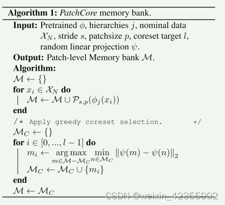
算法流程如下图所示

在这里插入图片描述

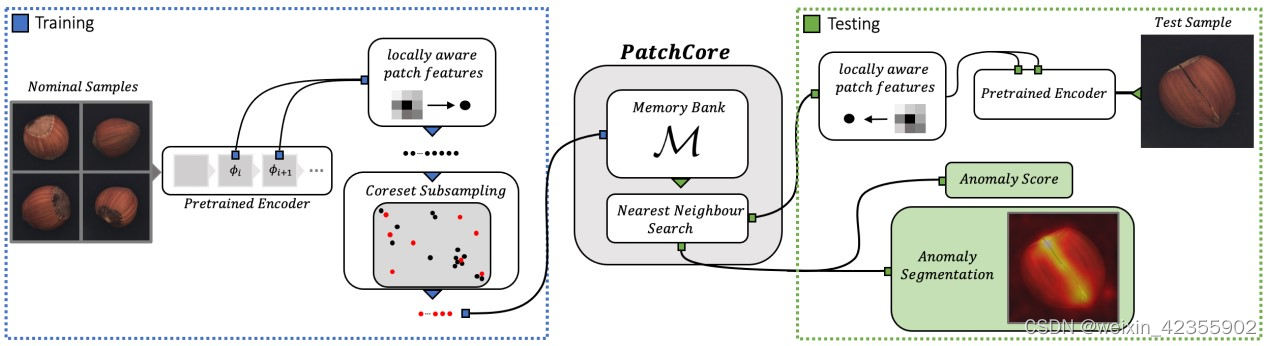
Locally aware patch features

imgs经过归一化后，images(2,3,224,224)
#提出layer2,layer3的输出，，[(2,512,28,28), (2,1024,14,14）]
 features = self.forward_modules["feature_aggregator"](images)

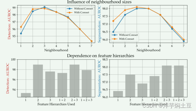
为什么选择layer2,layer3，下图中进行了对比

在这里插入图片描述

通过在局部邻域上进行特征聚合的方式来提取特征，作者p取3，这里 $\mathcal{N}_{p}^{(h,w)}$ 表示特征图上位置 (h,w)(ℎ,𝑤) 处大小为 p×p𝑝×𝑝 的一块patch

$\mathcal{N}_{p}^{(h,w)}=\{(a,b)|a\in[h-\lfloor p/2\rfloor,...,h+\lfloor p/2\rfloor],\\b\in[w-\lfloor p/2\rfloor,...,w+\lfloor p/2\rfloor]\},$

则位置 (h,w) 处的locally aware features如下:

$\phi_{i,j}\left(\mathcal{N}_{p}^{(h,w)}\right)=f_{\mathrm{agg}}\left(\{\phi_{i,j}(a,b)|(a,b)\in\mathcal{N}_{p}^{(h,w)}\}\right),$

文中，fagg表示邻域特征向量的聚合函数，使用adaptive average pooling自适应平均池。

#提取locally aware features
features = [self.patch_maker.patchify(x, return_spatial_info=True) for x in features]
# ->[(2, 784, 512, 3, 3),(2, 196, 1024, 3, 3)]
######################################################################
    #解析patchify作用
def patchify(self, features, return_spatial_info=False):
    """Convert a tensor into a tensor of respective patches.
    Args:
        x: [torch.Tensor, bs x c x w x h]
    Returns:
        返回patch，所有图像的patcch堆叠在一起
        x: [torch.Tensor, bs * w//stride * h//stride, c, patchsize,
        patchsize]
    """
    # 计算补丁的填充和展开，这里patch_size=3，stride=1，padding=1 ,28*28输出 28*28，torch.nn.Unfold 和卷积核差不多但是unfold是滑动到某一位置，直接取出输入张量中对应位置的值，然后flatten成一个一维向量，放到输出张量的对应位置处。(2,512,28,28)->(2,4608,784),其中4608=3*3*512，784=28x28。经过patchify提出的邻域特征表示维度分别为(2, 784, 512, 3, 3)、(2, 196, 1024, 3, 3)，其中784=28x28, 196=14x14。
    padding = int((self.patchsize - 1) / 2)
    unfolder = torch.nn.Unfold(
        kernel_size=self.patchsize, stride=self.stride, padding=padding, dilation=1
    ) 
    unfolded_features = unfolder(features) # (2,512,28,28)->(2,4608,784)
    # 计算补丁的数量，和卷积计算公式一样
    number_of_total_patches = []
    for s in features.shape[-2:]:  # (28,28)
        n_patches = (
                            s + 2 * padding - 1 * (self.patchsize - 1) - 1
                    ) / self.stride + 1
        number_of_total_patches.append(int(n_patches))  # (28,28)
    # 重塑未折叠特征张量
    unfolded_features = unfolded_features.reshape(
        *features.shape[:2], self.patchsize, self.patchsize, -1
    )  # (2,512,3,3,784)
    unfolded_features = unfolded_features.permute(0, 4, 1, 2, 3)  # (2,784,512,3,3)

    if return_spatial_info:  # True，则返回unfolded_features和补丁数量,否则只返回unfolded_features。
        return unfolded_features, number_of_total_patches
    return unfolded_features

由于features的维度[(2, 784, 512, 3, 3),(2, 196, 1024, 3, 3)]不一致，需要对layer3的输出进行bilinear插值使之与layer2匹配，

features = [features[layer] for layer in self.layers_to_extract_from]
features = [
    self.patch_maker.patchify(x, return_spatial_info=True) for x in features
]  # [(2, 784, 512, 3, 3),(2, 196, 1024, 3, 3)]
patch_shapes = [x[1] for x in features]  #
features = [x[0] for x in features]
ref_num_patches = patch_shapes[0]
# 对layer3的输出以匹配layer3的补丁数量
for i in range(1, len(features)):
    _features = features[i]
    patch_dims = patch_shapes[i]

    # TODO(pgehler): Add comments
    _features = _features.reshape(
        _features.shape[0], patch_dims[0], patch_dims[1], *_features.shape[2:]
    )  # (2, 14,14 , 1024, 3, 3)
    _features = _features.permute(0, -3, -2, -1, 1, 2)  # (2,1024, 3, 3,14,14 )
    perm_base_shape = _features.shape
    _features = _features.reshape(-1, *_features.shape[-2:])  # ( 18432,14,14)
    _features = F.interpolate(
        _features.unsqueeze(1),
        size=(ref_num_patches[0], ref_num_patches[1]),
        mode="bilinear",
        align_corners=False,
    )  # 对layer3进行线性插值-> ( 18432,28,28)
    _features = _features.squeeze(1)
    _features = _features.reshape(
        *perm_base_shape[:-2], ref_num_patches[0], ref_num_patches[1]
    )  # ->(2, 1024, 3, 3, 28, 28)
    _features = _features.permute(0, -2, -1, 1, 2, 3)  #
    _features = _features.reshape(len(_features), -1, *_features.shape[-3:])
    features[i] = _features  # (2, 784, 1024, 3, 3)
features = [x.reshape(-1, *x.shape[-3:]) for x in features]  # ->(1568, 512, 3, 3), (1568, 1024, 3, 3)

然后通过自适应平均池化进行特征聚合，即fagg：训练模型输出feature map上的每个位置(h, w)，都得到一个预先设定维度 d= 1024的单一表示，这样这样layer2、layer3的聚合特征[(1568, 512, 3, 3), (1568, 1024, 3, 3)]经过预处理，即分别经过自适应均值池化然后stack一起得到 (1568,2,1024)的输出特征。

features = self.forward_modules["preprocessing"](features)#  (1568,2,1024)
######################################################################
# 解析adaptive_avg_pool1d 池化聚合
class MeanMapper(torch.nn.Module):
    def __init__(self, preprocessing_dim):
        super(MeanMapper, self).__init__()
        self.preprocessing_dim = preprocessing_dim
 
    def forward(self, features):
        features = features.reshape(len(features), 1, -1)  # (1568,512,3,3)->(1568,1,4608)
        return F.adaptive_avg_pool1d(features, self.preprocessing_dim).squeeze(1)  # (1568,1,4608)->(1568,1024)
 
 
class Preprocessing(torch.nn.Module):
    def __init__(self, input_dims, output_dim):
        super(Preprocessing, self).__init__()
        self.input_dims = input_dims  # [512,1024]
        self.output_dim = output_dim  # 1024
 
        self.preprocessing_modules = torch.nn.ModuleList()
        for input_dim in input_dims:
            module = MeanMapper(output_dim)
            self.preprocessing_modules.append(module)
 
    def forward(self, features):  # [(1568,512,3,3),(1568,1024,3,3)]
        _features = []
        for module, feature in zip(self.preprocessing_modules, features):
            _features.append(module(feature))  # [(1568,1024),(1568,1024)]
        return torch.stack(_features, dim=1)  # (1568,2,1024)

再进一步进行特征聚合

features = self.forward_modules["preadapt_aggregator"](features)# (1568,1024)
######################################################################
#解析adaptive_avg_pool1d 池化聚合
class Aggregator(torch.nn.Module):
    def __init__(self, target_dim):
        super(Aggregator, self).__init__()
        self.target_dim = target_dim

    def forward(self, features):
        """Returns reshaped and average pooled features."""
        # batchsize x number_of_layers x input_dim -> batchsize x target_dim
        features = features.reshape(len(features), 1, -1) # (1568,2,1024)->(1568,1,2048)
        features = F.adaptive_avg_pool1d(features, self.target_dim)# (1568,1,1024)
        return features.reshape(len(features), -1)# (1568,1024)

features = np.concatenate(features, axis=0) #  得到训练集的所有feature。per batch两张图片的输出为(1568, 1024)，100张图片features map即为 (50 * 1568，1024)，这样就提出了提取locally aware features, 这里locally aware，是patch的p=3，1568= 2*(smoothing num:28*28)

Coreset-reduced patch-feature memory bank

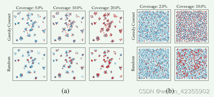
很显然随着图片的增多，features的增大，memory bank也变得越来越大，所以需要进行降采样，本文中选择 Greedy Coreset进行降采样(文中对比了随机降采样)，即每次选取离核心集最远的点加入核心集：

在这里插入图片描述

下图对比了降采样率效果：

在这里插入图片描述

features = self.featuresampler.run(features)
######################################################################
#解析
def run(
    self, features: Union[torch.Tensor, np.ndarray]
) -> Union[torch.Tensor, np.ndarray]:
    """Subsamples features using Greedy Coreset.

    Args:
        features: [N x D]
    """
    if self.percentage == 1: # 代码选取了降采样率为0.1
        return features
    self._store_type(features)
    if isinstance(features, np.ndarray):
        features = torch.from_numpy(features)
    reduced_features = self._reduce_features(features) # 为了寻找核心集速度（78400，1024）->(78400，128)
    sample_indices = self._compute_greedy_coreset_indices(reduced_features)# 通过 Greedy Coreset寻找核心集的索引
    features = features[sample_indices] # 降采样 （78400，1024）->(7840，1024)
    return self._restore_type(features)

def _reduce_features(self, features):
    if features.shape[1] == self.dimension_to_project_features_to:
        return features
    mapper = torch.nn.Linear(
        features.shape[1], self.dimension_to_project_features_to, bias=False
    ) # 通过线性映射WX 降低d的维度减少内存占用
    _ = mapper.to(self.device)
    features = features.to(self.device)
    return mapper(features)

 def _compute_greedy_coreset_indices(self, features: torch.Tensor) -> np.ndarray:
        """Runs approximate iterative greedy coreset selection.
		近似的贪心核心集选择算法，减少内存需求但增加了采样时间。
        This greedy coreset implementation does not require computation of the
        full N x N distance matrix and thus requires a lot less memory, however
        at the cost of increased sampling times.

        Args:
            features: [NxD] input feature bank to sample.
        """
        number_of_starting_points = np.clip(
            self.number_of_starting_points, None, len(features)
        )
        start_points = np.random.choice(
            len(features), number_of_starting_points, replace=False
        ).tolist()# 随机选择十个点
        approximate_distance_matrix = self._compute_batchwise_differences(
            features, features[start_points]
        )#所有feature与这10个features的距离，得到近似的距离矩阵，这是一种内存效率更高的方法，因为它避免了计算完整的 N x N 距离矩阵。
        #
        approximate_coreset_anchor_distances = torch.mean(
            approximate_distance_matrix, axis=-1
        ).reshape(-1, 1)
        coreset_indices = []
        num_coreset_samples = int(len(features) * self.percentage)

        with torch.no_grad():
            for _ in tqdm.tqdm(range(num_coreset_samples), desc="Subsampling..."):
                select_idx = torch.argmax(approximate_coreset_anchor_distances).item() # 与这10个features的最远的feature
                coreset_indices.append(select_idx)
                coreset_select_distance = self._compute_batchwise_differences(
                    features, features[select_idx : select_idx + 1]  # noqa: E203
                )#  其他feature与此feature的距离
                approximate_coreset_anchor_distances = torch.cat(
                    [approximate_coreset_anchor_distances, coreset_select_distance],
                    dim=-1,
                )
                approximate_coreset_anchor_distances = torch.min(
                    approximate_coreset_anchor_distances, dim=1
                ).values.reshape(-1, 1)

        return np.array(coreset_indices)
    
    
    def _compute_greedy_coreset_indices(self, features: torch.Tensor) -> np.ndarray:
        """Runs iterative greedy coreset selection.
				完整的贪心核心集选择算法
        Args:
            features: [NxD] input feature bank to sample.
        """
        distance_matrix = self._compute_batchwise_differences(features, features)
        coreset_anchor_distances = torch.norm(distance_matrix, dim=1)# 每个feature和其他feature的距离的sum

        coreset_indices = []
        num_coreset_samples = int(len(features) * self.percentage)

        for _ in range(num_coreset_samples):  # 每次迭代选择距离最远的样本加入核心集，并更新核心集锚点距离
            select_idx = torch.argmax(coreset_anchor_distances).item() #选出和其他feature最远的那个feature的index
            coreset_indices.append(select_idx)# 添加索引

            coreset_select_distance = distance_matrix[
                                      :, select_idx: select_idx + 1  # noqa E203
                                      ]# 其他feature与此feature的距离
            coreset_anchor_distances = torch.cat(
                [coreset_anchor_distances.unsqueeze(-1), coreset_select_distance], dim=1
            )
            coreset_anchor_distances = torch.min(coreset_anchor_distances, dim=1).values# 更新每个特征与所有已选择的核心集特征的最小距离。
		# 这样每次都更新coreset_anchor_distances中每个feature与核心集的最短距离
        return np.array(coreset_indices)

Anomaly Detection with PatchCore

代码中使用faiss实现knn搜索

self.anomaly_scorer.fit(detection_features=[features]) # Faiss实现最近邻检索和距离计算
##########################################
#解析
def _create_index(self, dimension):
    if self.on_gpu:
        return faiss.GpuIndexFlatL2(
            faiss.StandardGpuResources(), dimension, faiss.GpuIndexFlatConfig()
        )
    return faiss.IndexFlatL2(dimension) #创建索引
    
def fit(self, features: np.ndarray) -> None:
    """
    Adds features to the FAISS search index.

    Args:
        features: Array of size NxD.
    """
    if self.search_index:
        self.reset_index()
    self.search_index = self._create_index(features.shape[-1]) # 创建索引
    self._train(self.search_index, features)
    self.search_index.add(features)# add vectors to the index

test image图像进行loacl features的提取，对于每个loacl features，计算其到memory bank最近邻特征的距离作为异常得分，reshape在进行线性插值得到最后的热力图。在代码实现中，没有使用到公式7。公式7表明，若memory bank中对应最近的feature已经是memory bank中比较孤立的，需要乘上一个scale以增加其异常分数，个人认为代码没做的原因是需要对memory bank中的每个feature再算b个k近邻，增加了时间开销而没有实现

在这里插入图片描述
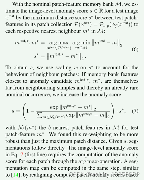
公式6，评估异常分数S，代码中S是test patch feature与memory bank中的最近的1个feature的距离作为异常分数
PS：不知道公式中的最大体现在，个人理解是如果没有进行降采样，memory bank每个聚类中有很多个feature，这样就要选取离这个聚类中最远那一个的距离作为异常分数，而降采样后每个feature就是一个聚类

_scores, _masks = self._predict(image) # image：输入图像，_scores：异常得分，_masks：(2,224,224)每轮test的heatmaps
#省略~~~ 循环结束后整合得到segmentations
min_scores = (
    segmentations.reshape(len(segmentations), -1)
    .min(axis=-1)
    .reshape(-1, 1, 1, 1)
)#(196,224,224)中的最小值
max_scores = (
    segmentations.reshape(len(segmentations), -1)
    .max(axis=-1)
    .reshape(-1, 1, 1, 1)
)
segmentations = (segmentations - min_scores) / (max_scores - min_scores) #(196,224,224) 对整个数据归一化，得到整test的heatmaps
################################################
#解析self._predict
# 对test image预测
def _predict(self, images):
    """Infer score and mask for a batch of images."""
    images = images.to(torch.float).to(self.device)
    _ = self.forward_modules.eval()

    batchsize = images.shape[0] # 2 
    with torch.no_grad():
        features, patch_shapes = self._embed(images, provide_patch_shapes=True) # 提取local features, 其中1568=2x28x28， 28x28是patch平滑取值的次数
        features = np.asarray(features) # (1568,1024)

        patch_scores = image_scores = self.anomaly_scorer.predict([features])[0] #(1568,1) 对于每个查询特征，计算其到最近邻特征的距离作为异常得分
        image_scores = self.patch_maker.unpatch_scores(
            image_scores, batchsize=batchsize
        ) # (1568,) -> ( 2, 784)
        image_scores = image_scores.reshape(*image_scores.shape[:2], -1) #( 2, 784) ->( 2, 784 ,1 )
        image_scores = self.patch_maker.score(image_scores)

        patch_scores = self.patch_maker.unpatch_scores(
            patch_scores, batchsize=batchsize
        ) # # (1568,) -> ( 2, 784)
        scales = patch_shapes[0] # (28,28)
        patch_scores = patch_scores.reshape(batchsize, scales[0], scales[1]) # ( 2, 28,28 )

        masks = self.anomaly_segmentor.convert_to_segmentation(patch_scores) # 异常得分reshape线性插值  ( 2, 28,28 ) -> mask:( 2, 224,224 )，然后高斯滤波平滑噪声

    return [score for score in image_scores], [mask for mask in masks]
# 解析self.anomaly_scorer.predict
def predict(
    self, query_features: List[np.ndarray]
) -> Union[np.ndarray, np.ndarray, np.ndarray]:
    """Predicts anomaly score.

    Searches for nearest neighbours of test images in all
    support training images.

    Args:
         detection_query_features: [dict of np.arrays] List of np.arrays
             corresponding to the test features generated by
             some backbone network.
    """
	features = self.feature_merger.merge(
        query_features,
    )
    query_distances, query_nns = self.imagelevel_nn(query_features) # 这里k取为1，return：(1568,1),(1568,1) 返回查询的最近距离和索引
    anomaly_scores = np.mean(query_distances, axis=-1) #(1568,1) 对于每个查询特征，计算其到最近邻特征的距离作为异常得分。
    return anomaly_scores, query_distances, query_nns #

最后得到第i个test的热力图(196,224,224)->(i,224,224)，

洋芋焖土豆

关注

20
点赞
踩
28

收藏

觉得还不错? 一键收藏
0
评论
PatchCore代码详解 | Towards Total Recall in Industrial Anomaly Detection

在代码实现中，没有使用到公式7。然后通过自适应平均池化进行特征聚合，即fagg：训练模型输出feature map上的每个位置(h, w)，都得到一个预先设定维度 d= 1024的单一表示，这样这样layer2、layer3的聚合特征[(1568, 512, 3, 3), (1568, 1024, 3, 3)]经过预处理，即分别经过自适应均值池化然后stack一起得到 (1568,2,1024)的输出特征。最后得到第i个test的热力图(196,224,224)->(i,224,224)，
复制链接

扫一扫