HDL-localization原理与源码解读

参考链接：
1、原理解读；
2、源码解读；

负责组内的定位导航也已经有一段时间了，HDL定位也用了一段时间，大部分情况下效果也还不错。但对其原理还是不是很清晰，只是大概知道用ukf融合了imu数据和匹配用的是ndt。最近要求优化定位效果，做一些自己的东西，因此需要了解原理进行增删改查。特此学习并记录ＨＤＬ定位的原理及源码。

一，ＨＤＬ原理

ｈｄｌ的后端数据融合使用的UKF，与EKF相比较，UKF更好地拟合非线性的概率分布，而不是强行进行线性化，EKF由于要计算雅可比矩阵，更烧脑一些，UKF要对协方差矩阵做开方，也需要用到矩阵分解，两者计算量差不多。当然，如果一定要用EKF应该也能解决如今的低速定位问题。
　在hdl中使用的ndt就像我们熟悉的pcl接口一样，只不过调用了多线程omp模式，它提供的是测量值。imu提供的是先验值，我们如果选择不用imu则先验值为原有的位姿。
　　参与融合的状态向量依然是p、v、q、ba、bg，一共16维，观测量则是7维，即p、q。和其它KF的接口一样，这里提供了predict和correct两个接口：
1.更新预测
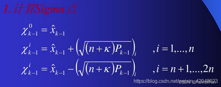
control是传入的一帧imu数据，我们姑且看作是控制量，预测时首先判断协方差矩阵是否是方阵并且是否正定，因为我们在求sigma点的过程中要求协方差矩阵的逆，因此提取出它们的特征值和特征向量并再次相乘。接下来就是求解sigma点了：

void computeSigmaPoints(const VectorXt& mean, const MatrixXt& cov, MatrixXt& sigma_points) {
    const int n = mean.size();
    assert(cov.rows() == n && cov.cols() == n);
    //用llt分解求协方差的逆矩阵
    Eigen::LLT<MatrixXt> llt;
    llt.compute((n + lambda) * cov);
    MatrixXt l = llt.matrixL();
 
    sigma_points.row(0) = mean;
    for (int i = 0; i < n; i++) {
      sigma_points.row(1 + i * 2) = mean + l.col(i);
      sigma_points.row(1 + i * 2 + 1) = mean - l.col(i);
    }
  }

在计算到所有的sigma点之后，用这些点重新拟合一个正态分布，在这个过程中引入了权重weights，它的初始赋值在构造函数中：

weights[0] = lambda / (N + lambda);
    for (int i = 1; i < 2 * N + 1; i++) {
      weights[i] = 1 / (2 * (N + lambda));
    }

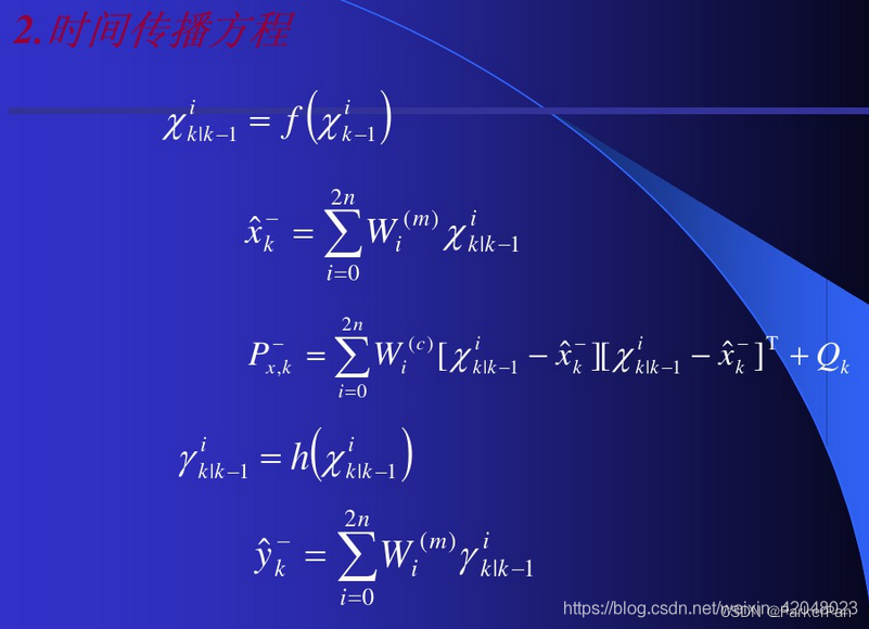
 void predict(const VectorXt& control) 
  {
    // calculate sigma points
    ensurePositiveFinite(cov);
    computeSigmaPoints(mean, cov, sigma_points);
    for (int i = 0; i < S; i++) {
      //状态转移方程
      sigma_points.row(i) = system.f(sigma_points.row(i), control);
    }
 
    const auto& R = process_noise;
 
    // unscented transform
    VectorXt mean_pred(mean.size());
    MatrixXt cov_pred(cov.rows(), cov.cols());
 
    mean_pred.setZero();
    cov_pred.setZero();
    for (int i = 0; i < S; i++) {
      mean_pred += weights[i] * sigma_points.row(i);
    }
    for (int i = 0; i < S; i++) {
      VectorXt diff = sigma_points.row(i).transpose() - mean_pred;
      cov_pred += weights[i] * diff * diff.transpose();
    }
    cov_pred += R;
 
    mean = mean_pred;
    cov = cov_pred;
  }

在每帧imu传入后都进行一次预测更新，在观测矫正之前我们得到了sigma点拟合的状态分布，而非状态转换矩阵，很像粒子滤波。

2.观测值估计真值

correct函数是观测矫正的过程，我们先拟合观测的sigma点，再用观测方程求解观测的均值，并加权计算扩增后的预测状态以及观测状态的协方差矩阵。

void correct(const VectorXt& measurement) 
  {
    // create extended state space which includes error variances
    //状态扩增，即先更新预测值的协方差矩阵，将上一部分用sigma点拟合的协方差加上测量噪声
    VectorXt ext_mean_pred = VectorXt::Zero(N + K, 1);
    MatrixXt ext_cov_pred = MatrixXt::Zero(N + K, N + K);
    ext_mean_pred.topLeftCorner(N, 1) = VectorXt(mean);
    ext_cov_pred.topLeftCorner(N, N) = MatrixXt(cov);
    ext_cov_pred.bottomRightCorner(K, K) = measurement_noise;
    //拟合状态扩增后的均值与协方差，也就是再算一遍sigma点
    ensurePositiveFinite(ext_cov_pred);
    computeSigmaPoints(ext_mean_pred, ext_cov_pred, ext_sigma_points);
 
    // unscented transform
    //UT变换，即拟合测量的均值和协方差
    expected_measurements.setZero();
    for (int i = 0; i < ext_sigma_points.rows(); i++) {
      expected_measurements.row(i) = system.h(ext_sigma_points.row(i).transpose().topLeftCorner(N, 1));
      expected_measurements.row(i) += VectorXt(ext_sigma_points.row(i).transpose().bottomRightCorner(K, 1));
    }
    //虽然叫expected，但这是7维的测量值，也就是用sigma点拟合的测量分布！
    VectorXt expected_measurement_mean = VectorXt::Zero(K);
    for (int i = 0; i < ext_sigma_points.rows(); i++) {
      expected_measurement_mean += ext_weights[i] * expected_measurements.row(i);
    }
    //测量的协方差矩阵，即Pk+1
    MatrixXt expected_measurement_cov = MatrixXt::Zero(K, K);
    for (int i = 0; i < ext_sigma_points.rows(); i++) {
      VectorXt diff = expected_measurements.row(i).transpose() - expected_measurement_mean;
      expected_measurement_cov += ext_weights[i] * diff * diff.transpose();
    }
 
    // calculated transformed covariance
    //那么，在这里的23*7的sigma矩阵就是状态扩增后的Pk|k+1
    MatrixXt sigma = MatrixXt::Zero(N + K, K);
    for (int i = 0; i < ext_sigma_points.rows(); i++) {
      auto diffA = (ext_sigma_points.row(i).transpose() - ext_mean_pred);
      auto diffB = (expected_measurements.row(i).transpose() - expected_measurement_mean);
      sigma += ext_weights[i] * (diffA * diffB.transpose());
    }
    //计算卡尔曼增益K=Pk|k+1/Pk
    kalman_gain = sigma * expected_measurement_cov.inverse();
    const auto& K = kalman_gain;
    //更新观测后的真值估计
    VectorXt ext_mean = ext_mean_pred + K * (measurement - expected_measurement_mean);
    MatrixXt ext_cov = ext_cov_pred - K * expected_measurement_cov * K.transpose();
 
    mean = ext_mean.topLeftCorner(N, 1);
    cov = ext_cov.topLeftCorner(N, N);
  }

最后简单总结一下UKF的过程：

1.产生2n+1个sigma点，在状态向量的附近，有点像粒子滤波。

2.利用状态转移矩阵，预测观测量的sigma点，并根据权重计算状态向量的均值和协方差矩阵。

3.利用测量矩阵得到sigma点的预测测量值。

4.根据sigma点和权重得到状态向量的预测值。

5.根据KF公式，将状态向量的预测值和观测值进行真值估计。

因此hdl的逻辑就很清晰地显示出来了，在获取到估计值后，便将状态向量的前10维，也就是pvq取出得到位姿的估计值，实现了定位的迭代。

  Eigen::Vector3f pos() const {
    return Eigen::Vector3f(ukf->mean[0], ukf->mean[1], ukf->mean[2]);
  }
 
  Eigen::Vector3f vel() const {
    return Eigen::Vector3f(ukf->mean[3], ukf->mean[4], ukf->mean[5]);
  }
 
  Eigen::Quaternionf quat() const {
    return Eigen::Quaternionf(ukf->mean[6], ukf->mean[7], ukf->mean[8], ukf->mean[9]).normalized();
  }
 
  Eigen::Matrix4f matrix() const {
    Eigen::Matrix4f m = Eigen::Matrix4f::Identity();
    m.block<3, 3>(0, 0) = quat().toRotationMatrix();
    m.block<3, 1>(0, 3) = pos();
    return m;
  }

二、源代码解析

主要参考：https://blog.csdn.net/wyang9x/article/details/112464644；
点云数据的预处理：
一般下面这几种情况需要进行点云滤波处理：

（1）点云数据密度不规则需要平滑

（2）因为遮挡等问题造成离群点需要去除

（3）大量数据需要下采样

（4）噪声数据需要去除
前文提到ＨＤＬ采用的是ｎｄｔ进行匹配的，单其实代码里是有GICP_OMP（广义迭代最近点）可选的

  void initialize_params() {
    // intialize scan matching method
    double downsample_resolution = private_nh.param<double>("downsample_resolution", 0.1);
    std::string ndt_neighbor_search_method = private_nh.param<std::string>("ndt_neighbor_search_method", "DIRECT7");

    double ndt_resolution = private_nh.param<double>("ndt_resolution", 1.0);
    boost::shared_ptr<pcl::VoxelGrid<PointT>> voxelgrid(new pcl::VoxelGrid<PointT>());
    voxelgrid->setLeafSize(downsample_resolution, downsample_resolution, downsample_resolution);
    downsample_filter = voxelgrid;
	//定义了ndt和glcp
    pclomp::NormalDistributionsTransform<PointT, PointT>::Ptr ndt(new pclomp::NormalDistributionsTransform<PointT, PointT>());
    pclomp::GeneralizedIterativeClosestPoint<PointT, PointT>::Ptr gicp(new pclomp::GeneralizedIterativeClosestPoint<PointT, PointT>());
	//ndt参数与搜索方法。默认DIRECT7，作者说效果不好可以尝试改为DIRECT1.
    ndt->setTransformationEpsilon(0.01);
    ndt->setResolution(ndt_resolution);
    if(ndt_neighbor_search_method == "DIRECT1") {
      NODELET_INFO("search_method DIRECT1 is selected");
      ndt->setNeighborhoodSearchMethod(pclomp::DIRECT1);
      registration = ndt;
    } else if(ndt_neighbor_search_method == "DIRECT7") {
      NODELET_INFO("search_method DIRECT7 is selected");
      ndt->setNeighborhoodSearchMethod(pclomp::DIRECT7);
      registration = ndt;
    } else if(ndt_neighbor_search_method == "GICP_OMP"){
    //GICP_OMP　需要在启动文件中的配置参数中配置；
      NODELET_INFO("search_method GICP_OMP is selected");
      registration = gicp;
    }
     else {
      if(ndt_neighbor_search_method == "KDTREE") {
        NODELET_INFO("search_method KDTREE is selected");
      } else {
        NODELET_WARN("invalid search method was given");
        NODELET_WARN("default method is selected (KDTREE)");
      }
      ndt->setNeighborhoodSearchMethod(pclomp::KDTREE);
      registration = ndt;
    }
    
    // initialize pose estimator
    //设置起点用。
    if(private_nh.param<bool>("specify_init_pose", true)) {
      NODELET_INFO("initialize pose estimator with specified parameters!!");
      pose_estimator.reset(new hdl_localization::PoseEstimator(registration,
        ros::Time::now(),
        Eigen::Vector3f(private_nh.param<double>("init_pos_x", 0.0), private_nh.param<double>("init_pos_y", 0.0), private_nh.param<double>("init_pos_z", 0.0)),
        Eigen::Quaternionf(private_nh.param<double>("init_ori_w", 1.0), private_nh.param<double>("init_ori_x", 0.0), private_nh.param<double>("init_ori_y", 0.0), private_nh.param<double>("init_ori_z", 0.0)),
        private_nh.param<double>("cool_time_duration", 0.5)
      ));
    }
  }

launch文件的更改：

<?xml version="1.0"?>
<launch>
  <!-- arguments -->
  <arg name="nodelet_manager" default="velodyne_nodelet_manager" />
  <arg name="points_topic" default="/velodyne_points" />
  <!-- input clouds are transformed in odom_child_frame, and then localization is performed in that frame -->
  <!-- this is useful to match the LIDAR and IMU coodinate systems -->
  <arg name="odom_child_frame_id" default="velodyne" />

  <!-- optional arguments -->
  <arg name="use_imu" default="false" />
  <arg name="invert_imu_acc" default="false" />
  <arg name="invert_imu_gyro" default="false" />
  <arg name="use_global_localization" default="true" />
  <arg name="imu_topic" default="/imu/data" />
  <arg name="enable_robot_odometry_prediction" value="false" />
  <arg name="robot_odom_frame_id" value="odom" />
  <arg name="plot_estimation_errors" value="false" />

  <include file="$(find hdl_global_localization)/launch/hdl_global_localization.launch" if="$(arg use_global_localization)" />

  <!-- in case you use velodyne_driver, comment out the following line -->
  <node pkg="nodelet" type="nodelet" name="$(arg nodelet_manager)" args="manager" output="screen"/>

    <!-- globalmap_server_nodelet -->
    <node pkg="nodelet" type="nodelet" name="globalmap_server_nodelet" args="load hdl_localization/GlobalmapServerNodelet $(arg nodelet_manager)">
      <param name="globalmap_pcd" value="$(find hdl_localization)/data/map.pcd" />
      <param name="convert_utm_to_local" value="true" />
      <param name="downsample_resolution" value="0.1" />
    </node>

    <!-- hdl_localization_nodelet -->
    <node pkg="nodelet" type="nodelet" name="hdl_localization_nodelet" args="load hdl_localization/HdlLocalizationNodelet $(arg nodelet_manager)">
      <remap from="/velodyne_points" to="$(arg points_topic)" />
      <remap from="/gpsimu_driver/imu_data" to="$(arg imu_topic)" />
      <!-- odometry frame_id -->
      <param name="odom_child_frame_id" value="$(arg odom_child_frame_id)" />
      <!-- imu settings -->
      <!-- during "cool_time", imu inputs are ignored -->
      <param name="use_imu" value="$(arg use_imu)" />
      <param name="invert_acc" value="$(arg invert_imu_acc)" />
      <param name="invert_gyro" value="$(arg invert_imu_gyro)" />
      <param name="cool_time_duration" value="2.0" />
      <!-- robot odometry-based prediction -->
      <param name="enable_robot_odometry_prediction" value="$(arg enable_robot_odometry_prediction)" />
      <param name="robot_odom_frame_id" value="$(arg robot_odom_frame_id)" />
      <!-- ndt settings -->
      <!-- available reg_methods: NDT_OMP, NDT_CUDA_P2D, NDT_CUDA_D2D-->
      <param name="reg_method" value="NDT_OMP" />
      
      <!-- if NDT is slow for your PC, try DIRECT1 serach method, which is a bit unstable but extremely fast -->
      <!--param name="ndt_neighbor_search_method" value="DIRECT1 " --/>
      <param name="ndt_neighbor_search_method" value="GICP_OMP" />
      <param name="ndt_neighbor_search_radius" value="2.0" />
      <param name="ndt_resolution" value="1.0" />
      <param name="downsample_resolution" value="0.1" />
      <!-- if "specify_init_pose" is true, pose estimator will be initialized with the following params -->
      <!-- otherwise, you need to input an initial pose with "2D Pose Estimate" on rviz" -->
      <param name="specify_init_pose" value="true" />
      <param name="init_pos_x" value="0.0" />
      <param name="init_pos_y" value="0.0" />
      <param name="init_pos_z" value="0.0" />
      <param name="init_ori_w" value="1.0" />
      <param name="init_ori_x" value="0.0" />
      <param name="init_ori_y" value="0.0" />
      <param name="init_ori_z" value="0.0" />

      <param name="use_global_localization" value="$(arg use_global_localization)" />
    </node>

    <node pkg="hdl_localization" type="plot_status.py" name="plot_estimation_errors" if="$(arg plot_estimation_errors)" />
</launch>