limma：单通道数据和RNA-seq数据差异性分析标准方法

前言

单通道数据极为流行，三大公司：Affymetrix、Illumina和Agilent的微阵列（microarray）技术产生的很多都是单通道数据。现在的主力的高通量测序机所产生的也是单通道数据，所以只要是被voom标准化（包括了log转化）的RNA-seq数据都可以看作和microarray一样的数据[引用]。这是一个很重要很有用的概念，相信会帮到很多生物信息入门者：

RNA-seq data + voom标准化 = microarray data

分析单通道数据其实是最好理解的，和普通的线性回归或者方差分析几乎是一样的。与微阵列数据不同的是，单通道数据通常需要依赖对比，缺少内参，所以R中设计程序的适合没几个标准参数可以用。这一篇文章中，我们仅仅使用最简单的两组对比设计的示例来做最简单的差异性分析。

示例

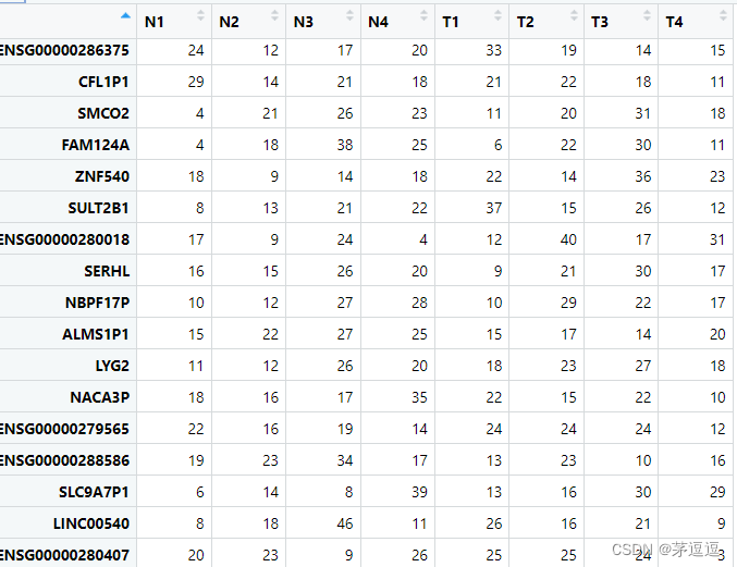
示例中的样本一共有两组共8个，前4个为正常组织，后4个为肿瘤组织。我们假设我们的表达举证为counts，counts应该长这样：

我们需要对这个矩阵进行voom转化，voom就是把 counts 转化为 log2-cpm的过程。

Voom

我们把下列的代码保存，并起名字为voom：

# assume counts is your Expression matrix
#Once a matrix of read counts counts has been created, with rows for genes and columns for samples,
#it is convenient to create a DGEList object using the edgeR package:

dge <- DGEList(counts=counts)

#The next step is to remove rows that consistently have zero or very low counts. One can for
#example use

keep <- filterByExpr(dge, design)
dge <- dge[keep,,keep.lib.sizes=FALSE]

# It is usual to apply scale normalization to RNA-seq read counts, and the TMM  normalization
#method in particular has been found to perform well in comparative studies. This can be applied
# to the DGEList object:
dge <- calcNormFactors(dge)



# voom 任选一种：
# 普通：
v <- voom(dge, design, plot=TRUE)
# 直接使用counts数据进行voom
# It is also possible to give a matrix of counts directly to voom without TMM normalization, by
v <- voom(counts, design, plot=TRUE)
# 如果你觉得原始数据噪声很大，也可以
#If the data are very noisy, one can apply the same between-array normalization methods as would
#be used for microarrays, for example:
v <- voom(counts, design, plot=TRUE, normalize="quantile")

设置分组

接下来就是设计矩阵了，根据要不要"对比矩阵"，我们得到type分配了分组（处理）：

type <- c("normal","normal","normal","normal","tumor","tumor","tumor","tumor")

设计矩阵分两种情况讨论

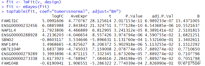
第一种：不要设计矩阵

# Here the first coefficient estimates the mean log-expression for wild type mice and plays the role
# of an intercept. 

Group <- factor(type, levels=c("normal","tumor"))
design <- model.matrix(~Group)
colnames(design) <- c("normal","tumorvsnormal")
design

source("voom")

fit <- lmFit(v, design)
fit <- eBayes(fit)
topTable(fit, coef="tumorvsnormal", adjust="BH")

 第二种：要设计矩阵

#第二种设计
#The second coefficient estimates the difference between mutant and wild type.
#Differentially expressed genes can be found by

design <- model.matrix(~0+type)
colnames(design) <- c("normal","tumor")

source("voom")

fit <- lmFit(v, design)
cont.matrix <- makeContrasts(tumorvsnormal=tumor-normal, levels=design)
fit2 <- contrasts.fit(fit, cont.matrix)
fit2 <- eBayes(fit2)
topTable(fit2, adjust="BH")

结果

我们看一下结果：

我们来看结果

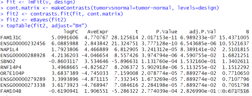
你会发现结果是一样的，以上是针对单通道数据和voom标化 RNA-seq数据而言的二组对比，也是最常用的差异性分析方法，分享给大家。 

引用

Law, C.W., Chen, Y., Shi, W., and Smyth, G.K. (2014). Voom: precision weights unlock linear model analysis tools for RNA-seq read counts. Genome Biology 15, R29