16S

Alpha diversity：种内，richness Chao1,evenness Shannon index.

• Alpha diversity
  • Shannon’s diversity index (a quantitative measure of community richness)
  • Observed OTUs (a qualitative measure of community richness)
  • Faith’s Phylogenetic Diversity (a qualitiative measure of community richness that incorporates phylogenetic relationships between the features)
  • Evenness (or Pielou’s Evenness; a measure of community evenness)
• Beta diversity
  • Jaccard distance (a qualitative measure of community dissimilarity)
  • Bray-Curtis distance (a quantitative measure of community dissimilarity)
  • unweighted UniFrac distance (a qualitative measure of community dissimilarity that incorporates phylogenetic relationships between the features)
  • weighted UniFrac distance (a quantitative measure of community dissimilarity that incorporates phylogenetic relationships between the features)

 

对于Faith’s phylogenitci diversity的理解。

在这个set/样本中PD=41,是树枝长度的总和，少掉一个分支，PD值就减少一个。体现了进化上的复杂度。

Chao1 is an estimator based on abundance. This means that the data it requires refer to the abundance of individuals belonging to a certain class in a sample. A sample is any list of species in a site, location, quadrant, country, unit of time, trap, etcetera. As we know, there are many species that are only represented by a few individuals in a sample (rare species), compared to the common species, which can be represented by numerous individuals. The Chao1 estimator is based on the presence of the former. That is, we need to know how many species are represented by only one individual in the sample (singletons), and how many species are represented by exactly two individuals (doubletons): Sest = Sobs + F2 / 2G, where: Sest is the number of classes ( in this case, number of species) that we want to know, Sobs is the number of species observed in a sample, F is the number of singletons and G is the number of doubletons. In the programEstimates a corrected formula has also been integrated for this model, which is applied when the number of doubletons is zero: Sest = Sobs + ((F2 / 2G + 1) - (FG / 2 (G + 1) 2)).

Chao2 is the estimator based on the incidence. This means that it needs presence-absence data of a species in a given sample, that is, only if the species is present and how many times is that species in the sample set: Sest = Sobs + (L2 / 2M), where: L is the number of species that occur only in one sample ("unique" species), and M is the number of species that occur in exactly two samples ("double" or "duplicate" species). For example, if we have a set of grids, we need to know how many species are in a grid and how many species are in two. The formula corrected in Estimates, which is applied when the number of doubles is zero, is: Sest = Sobs + ((L2 / 2M + 1) - (LM / 2 (M + 1) 2)). To use both estimators in ESTIMATES, data in the form of a matrix is ​​needed, where rows and columns can represent samples and species indistinctly; it is necessary to establish the order once the program has started. Estimates also allows the calculation of the standard deviation of the two estimators. Once several randomisations are made (50 recommended, but can be 100 or more), with or without replacement, and when the total number of samples has been used, the final value of the estimator is obtained and the results can be plotted. The number of samples is presented on the x axis, and the number of species in the dependent variable. Thus, the Sest and the Sobs can be compared. But the final graph is interpreted differently from the conventional one: when you have the total number of samples, there is a certain separation between the curve of the Sest and the Sobs. That separation would be indicating how many species are missing to register in that community. The more separated they are, we would expect that the total number of species that contains the place is greater than the one that we currently know.

For additional information please read the following chapter Estimating species richness in the following link:

https://www.uvm.edu/~ngotelli/manuscriptpdfs/Chapter%204.pdf

 

 Based on the OTUs, richness estimators (Ace and Chao) and diversity indices (Shannon and Simpson) were calculated for the samples within a 0.03 difference

Beta diversity: 种间，Bray-Curtis, UniFrac (依赖系统发育树，mothur，Qiime可得树) and weighted UniFrac distance

The Aitchison distance is a sub-compositionally coherent distance defined as the Euclidean distance after the clr-transformation of the compositions.

The goal of ordination plots is the visualization of beta diversity for identification of possible data structures.

PCA分析，PCoA分析二者的只要区别就是PCA采用了欧式距离，而PCoA采用其他距离。PCoA分析时，特征值不能是负数vegan and phyloseq俩包可以作图

非度量多维尺度分析（nonmetric multidimensional scaling, NMDS），是一种简介的梯度分析方法，也是基于距离或者相异性矩阵。与其它主要用于最大化变异和一致性的方法不一样，NMDS是一种排序方法。这对于距离缺失的数据有优势，只要先办法确定对象之间的位置关系，便可以进行NMDS分析

PERMANOVA [25], is perhaps the most widely used distance-based method for multivariate community analysis.

如果发现了差异，那么哪些群体是主因？ANCOM [35] and ALDEx2

The algorithm for the selection of microbial balances is implemented in the R package selbal

Co-occurrence network analysis, by Spearman’s correlation analysis and visualized using the Cytoscape software

Chao1 and ACE indices were used to estimate community richness, 群体丰富度

and the Shannon and phylogenetic diversity (PD) whole tree indices were applied to measure microbial diversity.

Good’s coverage was used to evaluate the coverage quality of sequencing results

 

Tax4fun功能预测

STAMP

Analysis of similarity (ANOSIM) and permutational multivariate analysis of variance (PERMANOVA) were performed to test the dissimilarity of beta diversity between groups by using ANOSIM and Adonis functions of vegan package in R

 

Linear discriminant analysis effect size (LEfSe) algorithm (Segata et al., 2011) was used to identify specific microbial taxa and functions that differed significantly between groups。 The analysis of differences in the abundance of the microbiota between two groups were also performed using the DESeq. 2 package in R。 寻找组间不同代表物种。

PCA和LDA的差别在于，PCA，它所作的只是将整组数据整体映射到最方便表示这组数据的坐标轴上，映射时没有利用任何数据内部的分类信息，是无监督的，而LDA是由监督的，增加了种属之间的信息关系后，结合显著性差异标准测试(克鲁斯卡尔-沃利斯检验和两两Wilcoxon测试)和线性判别分析的方法进行特征选择。

NMDS分析基于OUT level

Qualitative and quantitative comparison of the community composition at different levels of taxonomic organization (phylum, class, order, family) were carried out using Nonmetric Multidimensional Scaling - NMDS35 with Bray-Curtis distance metric36, Gower distance metric37 and Jaccard distance metric

 

Community richness and diversity were quantified using phylogenetic diversity (PD) (59) and Shannon and Simpson indices within QIIME 1.9.1. Differences in community composition were calculated using weighted and unweighted UniFrac metrics (60), with communities rarefied to 17,212 sequences per sample, and PCoA and nonmetric multidimensional scaling (NMDS) were performed with QIIME. Weighted and unweighted UniFrac distance matrices were strongly correlated (Mantel r 0.78, P  0.001), so ordination plots are presented only for unweighted Unifrac data. Statistical significance corresponding to differences in beta diversity across discrete sample groupings was calculated using ANOSIM, and correlations between weighted and unweighted UniFrac distance and continuous environmental variables were tested using Mantel’s r statistic. BEST analysis was used to find the highest Spearman’s correlation value for comparisons between community dissimilarities and groups of environmental variables (37) by selecting all possible subsets of environmental variables given by the user and scaling and calculating the Euclidean distances for each subset (37). Spearman’s correlation coefficients were calculated using R (Core Development Team 2015), and corresponding P values were adjusted to compensate for the false-discovery rate (FDR [ q]). Network analysis was performed on sample OTUs. Prior to analysis, rare OTUs with abundances of less than 0.01% of the total number of OTUs were removed, resulting in a final subset of 1,293 OTUs. Co-occurrence of OTUs was defined based on their Spearman correlations using the WGCNA package (61). The nodes in each network represent OTUs, and the edges connecting the nodes represent correlations between OTU pairs. All P values were adjusted for multiple testing using the Benjamini and Hochberg FDR controlling procedure (62), as implemented in the multtest R package. The directcorrelation dependencies were distinguished using the network deconvolution method (63). Edges were pruned to keep only high-correlation coefficients and significant FDR-adjusted P values for correlations. The cutoff for presenting FDR-adjusted P values was 0.01, and the cutoff of correlation coefficients was found to be 0.81 for the global network through the random matrix theory (RMT) method (58). Network statistical properties were calculated at the sample level with the igraph R package and aggregated at each climate level. Graphical representations for the subnetwork arid, margin, and hyperarid data had RMT thresholds of 0.82, 0.92, and 0.84, respectively

Some network statistics are impacted by community richness, and our three climate classes (arid, margin, and hyperarid) differ in their levels of community richness. We therefore tested our conclusions for robustness with respect to differences in richness by reducing our higher-richness samples (from the arid and margin sites) to the richness level of the hyperarid sites and recomputing our network statistics. The effect of richness reduction was tested by rarefying the initial OTU table 500 times to 300 reads per sample and removing rare OTUs using the same method as that described before. Networks were created and statistics were averaged across all 500 repeats using R

co-occurrence network interactions

co-exclusion network

Network construction
To reduce rare OTUs in the data set, we removed OTUs with relative abundances less than 0.01%
of the total number of archaeal, bacteria, and fungal sequences, respectively. The co-occurrence network was inferred based on the Spearman correlation matrix constructed with the WGCNA package (Langfelder and Horvath, 2012). The nodes in this network represent OTUs and the edges that connect these nodes represent correlations between OTUs. We adjusted all P-values for multiple testing using the Benjamini and Hochberg false discovery rate (FDR) controlling procedure (Benjamini et al., 2006), as implemented in the multtest R package. The direct correlation dependencies were distinguished using the network deconvolution method (Feizi et al.,
2013). Based on correlation coefficients and FDRadjusted P-values for correlation, we constructed cooccurrence networks. The cutoff of FDR-adjusted P-values was 0.001. The cutoff of correlation coefficients was determined as 0.78 through random matrix theory-based methods (Luo et al., 2006). Network properties were calculated with the igraph package. We generated network images with Gephi (http://gephi.github.io/). All samples were divided into groups by climatic region. The impact of each sample group on the Spearman correlation value of each edge in the network was assessed by dividing the omission score (OS) (Spearman correlation value without these samples) by the absolute original Spearman score (Lima Mendez et al., 2015). To account for group size, the OS was computed repeatedly for random, same-size sample sets. Nonparametric P-values were calculated as the number of times random OSs were smaller than the sample group OS, divided by the number of random Oss (500 for each taxon pair). Edges were classified as region-specific when the ratios of OSs to absolute original scores were below one and adjusted P-values were below 0.05.

 

Topological feature analysis
We calculated topological features (Supplementary Table S1) for each node in the network with
the igraph package (Csardi and Nepusz, 2006). This feature set included betweenness centrality (the number of shortest paths going through a node), closeness centrality (the number of steps required to access all other nodes from a given node), transitivity (the probability that the adjacent nodes of a node are connected, also called the clustering coefficient) and degree (the number of adjacent edges). The betweenness centrality feature was used to measure the centrality of each node in the network. Nodes were further classified as peripheral, intermediate or central by ranking all nodes according to centrality, partitioning this ranked list into three equally populated bins, which were termed ‘centrality tiers’ (Greenblum et al., 2012). Nodes with high degree (4100) and low betweenness centrality values (o5000) are recognized as keystone species in co-occurrence networks.

斯皮尔曼等级相关系数是反映两组变量之间联系的密切程度，它和相关系数r一样，取值在-1到+1之间，所不同的是它是建立在等级的基础上计算的, 斯皮尔曼等级相关对数据条件的要求没有积差相关系数严格，只要两个变量的观测值是成对的等级评定资料，或者是由连续变量观测资料转化得到的等级资料，不论两个变量的总体分布形态、样本容量的大小如何，都可以用斯皮尔曼等级相关来进行研究。它与样本的容量有关，尤其是在样本容量比较小的情况下，其变异程度较大，等级相关系数的显著性检验与普通的相关系数的显著性检验相同

群落谱系距离（phylogenetic distance）:群落I与群落II中种俩俩之间谱系分支长度之和的平均值, PD_whole_tree:sum of branch lengths between all representatives

goods_coverage  测序深度指数测序深度：C=1-n1/N,n1为只有含一条序列的OTU数目，N为抽样中出现的总的序列数目。

谱系多样性（phylogenetic diversity PD），某个地点所有物种间最短进化分支长度之和占各节点分支长度综合的比例

simpson  菌群多样性指数辛普森多样性指数=随机取样的两个个体属于不同种的概率=1-随机取样的两个个体属于同种的概率 越均匀，值越大

 

SparCC was developed to calculate correlations between OTU abundances in microbiome
data whilst accounting for their inherent sparsity and compositionality

CoNet is itself an ensemble approach. The package allows a range of co-occurrence measures to be combined with several options for how to combine the weighting of edges
and their p-values.

To complement these statistical techniques, we also compare healthy and diseased networks using mesoscale analytic techniques, which can offer insights into the structure of clusters of microbes that tend to co-occur with one another relatively consistently over individuals.

To assess similarity between the partitions of species into communities, we use the Rand index35, which is a statistical measure that quantifies similarities between partitions of items into sets.

To
infer correlations between OTUs and OTUs and environmental parameters, we first removed OTUs with a relative abundance below 0.1% of the total number of reads. We also removed all samples that had <7500 reads. Rare OTUs and samples with low sequencing depth might cause artifacts in the network analysis (Berry and Widder, 2014; Ju et al., 2014)

Ten iterations were used to estimate the median correlation of each pairwise and the statistical significance of the correlations was calculated by bootstrapping with 500 iterations. Correction for multiple-testing of the P values was performed in R according to Benjamini-Hochberg method. Correlations were then sorted for statistical significance (p < 0.05) and R > ±0.6

 

 

In order to account for the effect of indirect taxon edges driven by environmental parameters, methods from LimaMendez et al. (2015) were applied

在co-occurrence network中，网络中节点的相邻节点数越高，表示在该群体更高的共发生。

Statistical Analysis

Each experiment was independently triplicated to derive an average and standard deviation. Data were presented as mean ± SEM when indicated. T test was used for statistical analyses by Prism 7.0 (GraphPad Software Inc., USA). Differences were considered significant at P < 0.05. LEfSe [linear discriminant analysis (LDA) effect size] was applied to identify bacterial biomarkers. The LDA > 4.0 was set as the threshold for selection of features. The Wilcoxon rank-sum test was used to compare the crucial taxa between groups.

Ecological patterns of the human microbiota exhibit high inter-subject variation, with few operational taxonomic units (OTUs) shared across individuals. To overcome these issues, non-parametric approaches, such as the Mann-Whitney U-test and Wilcoxon rank-sum test, have often been used to identify OTUs associated with host diseases. However, these approaches only use the ranks of observed relative abundances, leading to information loss, and are associated with high false-negative rates. In this study, we propose a phylogenetic tree-based microbiome association test (TMAT) to analyze the associations between microbiome OTU abundances and disease phenotypes. Phylogenetic trees illustrate patterns of similarity among different OTUs, and TMAT provides an efficient method for utilizing such information for association analyses. The proposed TMAT provides test statistics for each node, which are combined to identify mutations associated with host diseases.

 

qiime dada2 denoise-paired
–i-demultiplexed-seqs ~/QIIME2_2_import/paired-end-demux.qza
–p-trim-left-f 13
–p-trim-left-r 13
–p-trunc-len-f 270
–p-trunc-len-r 270
–p-n-threads 0
–o-table ~/QIIME2_3_demux/table_540.qza
–o-representative-sequences ~/QIIME2_3_demux/rep-seqs_540.qza
–o-denoising-stats ~/QIIME2_3_demux/denoising-stats_540.qza

 

Thanks for your reply. I not looking for a demultiplexing method, I wanna know “how should I fill in the index information into the sample-metadata”, since for the dual-indexed suequences, the index 1 (in read 1) and index (in read 2) are different in sequence, for example, index 1 is ATCTGC, while index 2 is TTGCAG，and the QIIME2 uses the index 1: index 2 in sample-metadata.tsv to recognize the corresponding sequence. here I would like to know whether I need to fill the both indice in the sample-metadata. In the example of qiime tutorial, even if the sequences are dual-indexed, but the dual-index are the same, so in the sample-metadata, only one index sequence was filled out. Thanks a lot

Parameters:

  --m-forward-barcodes-file METADATA

  --m-forward-barcodes-column COLUMN  MetadataColumn[Categorical]

                          The sample metadata column listing the per-sample

                          barcodes for the forward reads.           [required]

  --m-reverse-barcodes-file METADATA

  --m-reverse-barcodes-column COLUMN  MetadataColumn[Categorical]

                          The sample metadata column listing the per-sample

You’ll need to set these 4 parameters for dual-index demultiplexing. The metadata file can be any metadata file you are using however it will have to have at least 3 columns, your sample-id, forward-index, and reverse-index. The column names for your indices can be whatever you want as long as it it matches the requirements here 5. so for example:

• q2-alignment # 生成和操作多序列比对
• q2-composition # 用于物种数据分析
• q2-cutadapt # 从序列数据中删除接头序列，引物和其他不需要的序列
• q2-dada2 # 序列质量控制
• q2-deblur # 序列质量控制
• q2-demux # 混池测序样本拆分和查看序列质量
• q2-diversity # 探索群落多样性
• q2-emperor # beta多样性3D可视化
• q2-feature-classifier # 物种注释
• q2-feature-table # 按条件操作特征表
• q2-fragment-insertion # 系统发育树扩展，确定准确的进化地位
• q2-gneiss # 构建组合模型
• q2-longitudinal # 成对样本和时间序列分析
• q2-metadata # 处理元数据
• q2-phylogeny # 生成和操纵系统发育树
• q2-quality-control # 用于特征和序列数据质量控制
• q2-quality-filter # 基于PHRED的过滤和修剪
• q2-sample-classifier # 样本元数据的机器学习预测
• q2-taxa # 处理特征物种分类注释
• q2-types # 定义微生物组分析的类型
• q2-vsearch # 聚类和去冗余
• QIIME默认的抽样方法是从第10个OUT代表序列开始，到第38895个OUT代表序列截止，其间抽样10次，每次增加3888条序列。因为每个样本总体中物种的序列是随机分布的，而且样本容量是从小到大逐步增加，所以在解读结果时一定要清楚以下几点：
• 1. 有可能样本总体中靠前的序列shannon指数和simpson指数均高于平均值，那么在图上会出现先下降再到平台区的曲线。
• 2. 各样本中OTU数不同，而随机抽样时有可能有些样品的总量达不到38895，因此在网页结果的表格中会有nan（即Not a Number）表示缺损，同时反映在图上是每个样品的曲线终点并不同一x轴位置。
• 3. 用样本总体算出来的多样性指数和这种抽样算出来的曲线终点位置有出入，只是位置接近，并不相等，这很正常。rarefaction曲线的意义是反应一种变化情况，其终点位置仅供参考。因为有些样本OUT代表序列多于38895，有些少于38895，而如果用所有序列计算得到的只是最后的一个值。
• Alpha rarefaction curve主要用于检测测序量是否充足。这里用到的方法是逐步扩大随机抽样的样本容量，如果样本容量扩大了但曲线再无变化（准确来讲，变化非常微小）时，则认为测序量已充足，再增加测序量，样本的alpha多样性指标也不会有太多的变化，即样本alpha多样性指标达到稳定。
   
• PD_whole_tree，chao1，observed_otus指标变化趋势相近，这一组反应的是样本中物种的丰度，均表现为前期增长快，后期增长慢，但是会随着样本容量的扩大而一直增加，因为样本容量增加时每个样本中OTU数会不断增加。
   
• shannon，simpson指标变化趋势相近，这一组反应的是样本中物种的多样性，均表现为前期快速改变，在某个点过后进入平台区。

多样性随物种丰富度和均匀度的增加而增加。Simpson指数兼顾丰富度和均匀度。

 

UniFrac分析利用各样品序列间的进化信息来比较环境样品在特定的进化谱系中是否有显著的微生物群落差异 UniFrac 可用于beta 多样性的评估分析，即对样品两两之间进行比较分析，得到样品间的unifrac距离矩阵。其计算方法为：首先利用来自不同环境样品的OTU 代表序列构建一个进化树，Unifrac 度量标准根据构建的进化树枝的长度计量两个不同环境样品之间的差异，差异通过0-1 距离值表示，进化树上最早分化的树枝之间的距离为1，即差异最大，来自相同环境的样品在进化树中会较大几率集中在相同的节点下，即它们之间的树枝长度较短，相似性高。若两个群落完全相同,那么它们没有各自独立的进化过程,UniFrac值为0;若两个群落在进化树中完全分开,即它们是完全独立的两个进化过程,那么UniFrac值为1。

从UniFrac的定义中,可以看出它只考虑序列是否在群落中出现,而不考虑序列的丰度。若两个群落包含的物种完全相同,那么不管每个物种的丰度是否有差别或者差别的大小，UniFrac值为0。weighted unifrac方法,就是在UniFrac的基础上,将序列的丰度纳入考虑,它能够区分物种丰度的差别。在计算中, weighted unifrac按照每条枝指向的叶节点中来自两个群落的比例,给每条枝加权重。因此unweighted unifrac 可以检测样品间变化的存在，而weighted unifrac 可以更进一步定量的检测样品间不同谱系上发生的变异。

(un)Weighted UniFrac 分析

(un)Weighted UniFrac 分析

UniFrac分析利用各样品序列间的进化信息来比较环境样品在特定的进化谱系中是否有显著的微生物群落差异。 UniFrac 可用于beta 多样性的评估分析，即对样品两两之间进行比较分析，得到样品间的unifrac距离矩阵。其计算方法为：首先利用来自不同环境样品的OTU 代表序列构建一个进化树，Unifrac 度量标准根据构建的进化树枝的长度计量两个不同环境样品之间的差异，差异通过0-1 距离值表示，进化树上最早分化的树枝之间的距离为1，即差异最大，来自相同环境的样品在进化树中会较大几率集中在相同的节点下，即它们之间的树枝长度较短，相似性高。若两个群落完全相同,那么它们没有各自独立的进化过程,UniFrac值为0;若两个群落在进化树中完全分开,即它们是完全独立的两个进化过程,那么UniFrac值为1。

从UniFrac的定义中,可以看出它只考虑序列是否在群落中出现,而不考虑序列的丰度。若两个群落包含的物种完全相同,那么不管每个物种的丰度是否有差别或者差别的大小，UniFrac值为0。weighted unifrac方法,就是在UniFrac的基础上,将序列的丰度纳入考虑,它能够区分物种丰度的差别。在计算中, weighted unifrac按照每条枝指向的叶节点中来自两个群落的比例,给每条枝加权重。因此unweighted unifrac 可以检测样品间变化的存在，而weighted unifrac 可以更进一步定量的检测样品间不同谱系上发生的变异。

 软件及算法：使用FastTree（version 2.1.3 http://www.microbesonline.org/fasttree/）根据最大似然法（ approximately-maximum-likelihood phylogenetic trees ） 构建进化树，然后利用Fastunifrac[2] （http://unifrac.colorado.edu/）分析得到样品间距离矩阵。 

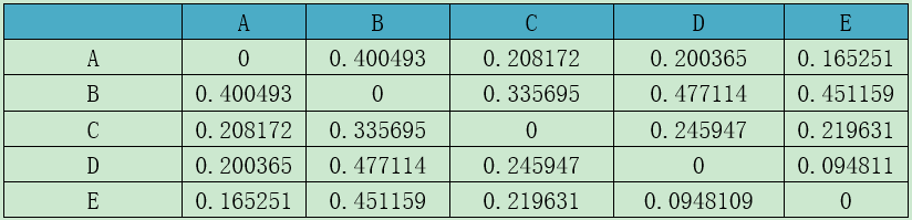
Table（un）weighted unifrac distance matrix

注：第一行和第一列均为样品。
参考文献：
　　[1] Tanya Yatsunenko, Federico, et al. Human gut microbiome viewed across age and geography. Nature486, 222–227 (14 June 2012) doi:10.1038.nature11053.
　　[2] Micah Hamady, Catherine Lozupone and Rob Knight. Fast UniFrac:facilitatinghigh-throughput phylogenetic analyses of microbial communities including analysis of pyrosequencing and PhyloChip data.The ISME Journal (2010) 4, 17–27; doi:10.1038/ismej.2009.97

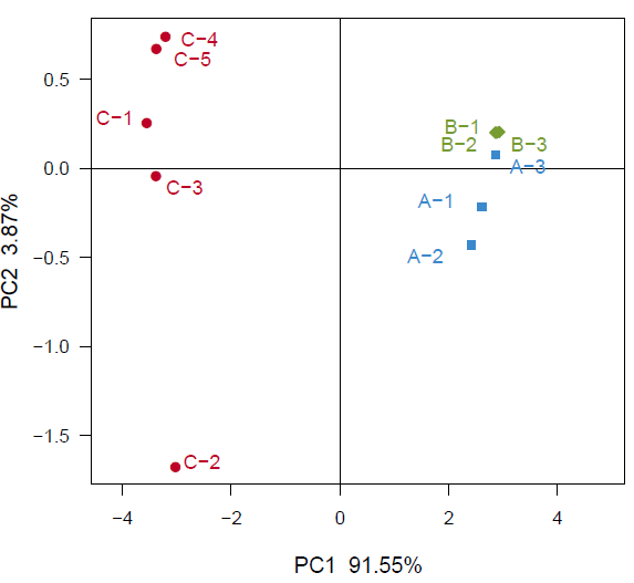
基于UniFrac 的Pcoa 分析

Unifrac 分析得到的距离矩阵可用于多种分析方法，可通过多变量统计学方法PCoA 分析，直观显示不同环境样品中微生物进化上的相似性及差异性。 PCoA（principal co-ordinates analysis）是一种研究数据相似性或差异性的可视化方法，通过一系列的特征值和特征向量进行排序后，选择主要排在前几位的特征值，PCoA 可以找到距离矩阵中最主要的坐标，结果是数据矩阵的一个旋转，它没有改变样品点之间的相互位置关系，只是改变了坐标系统。通过PCoA 可以观察个体或群体间的差异。
分析软件：R 语言PCoA 分析和作PCoA 图。
　　unifrac.pcoa.tiff :样品PCoA 分析图

Fig (un)weighted unifrac PCoA analysis

参考文献：
　　Xiao-Tao Jiang ,Xin Peng, et al.Illumina Sequencing of 16S rRNA Tag Revealed Spatial Variations of Bacterial Communities in a Mangrove Wetland. Microb Ecol (2013) 66:96–104.DOI10.1007/s00248-013-0238-8.
　　注：PC1 和PC2 是两个主坐标成分，PC1 表示尽可能最大解释数据变化的主坐标成分，PC2 为解释余下的变化度中占比例最大的主坐标成分，PC3 等依次类推。

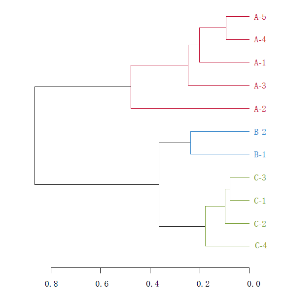
基于UniFrac 的多样品相似度树分析

Unifrac 分析得到的距离矩阵可用于多种分析方法，通过层次聚类（Hierarchical cluatering）[1]中的非加权组平均法UPGMA 构建进化树等图形可视化处理，可以直观显示不同环境样品中微生物进化上的相似性及差异性。
　　UPGMA（Unweighted pair group method with arithmetic mean）假设在进化过程中所有核苷酸/氨基酸都有相同的变异率，即存在着一个分子钟。通过树枝的距离和聚类的远近可以观察样品间的进化距离。
分析软件： R 语言vegan 包UPGMA 分析和作进化树。

(un) weighted unifrac tree analysis

(un) weighted unifrac tree analysis

注：树枝颜色为预先定义的不同分组标注。
参考文献：
　　[1] Magali Noval Rivas, PhD, Oliver T. Burton, et al. A microbita signature associated with experimental food allergy promotes allergic senitization and anaphylaxis. The Journal of Allergy and Clinical Immunology.Volume 131, Issue 1 , Pages 201-212, January 2013.

 

分级发育树

　　NCBI 提供了已有微生物物种的分类学信息数据库（ 数据库文件下载地址：ftp://ftp.ncbi.nih.gov/pub/taxonomy/），数据库中包含微生物的分类学系统关系树。在前述分类学分析中，已经得到了每个OTU 的丰度和对应的分类学信息，将测序得到的物种丰度信息回归至数据库的分类学系统关系树中，可以从整个分类系统上全面了解测序的环境样品中所有微生物的进化关系和丰度差异。

软件及方法：MEGAN（http://ab.inf.uni-tuebingen.de/software/megan/）。导入分析数据中样品包含的物种及物种丰度，通过交互式搜索NCBI 的分类数据库信息，以树状图形式表现物种的丰度情况和群落结构，反映微生物的组成情况，这种方法构建的系统树不同于利用序列碱基差异构建的系统发育树，不能反应物种间的时间进化信息。

单样本分类发育

 

多样本分类学发育树

Multi samples Taxonomy analysis tree

 

　注：图中的支点表示该处在NCBI 数据库中有相应的Taxonomy 记录，支点附近有该英文名称拼写。多个样品同时作图时，可在树枝或结点处通过小型饼状图以不同颜色表示不同样品的相对丰度差异。

环形发育树

　　系统发生进化树（环形发育树）

　　在分子进化研究中，系统发生的推断能够揭示出有关生物进化过程的顺序，了解生物进化历史和机制，可以通过序列间碱基的差异构建进化树。选择OTU的代表序列根据邻位比对法（neighbor-joining）构建进化树，结果可以用列图或者圈图的形式呈现。

　　使用软件：MEGA和iTOL（http://itol.embl.de/）

注：进化树中每条树枝代表一个物种，树枝长度为两个物种间的进化距离，即物种的差异程度。

RDA/CCA分析

　　RDA 或者CCA是基于对应分析发展而来的一种排序方法，将对应分析与多元回归分析相结合，每一步计算均与环境因子进行回归，又称多元直接梯度分析。此分析是主要用来反映菌群与环境因子之间关系。RDA是基于线性模型，CCA 是基于单峰模型。分析可以检测环境因子、样品、菌群三者之间的关系或者两两之间的关系。
　　RDA 或CCA 模型的选择原则：先用species-sample 数据（97%相似性的样品OTU 表）做DCA 分析，看分析结果中Lengths of gradient 的第一轴的大小，如果大于4.0，就应该选CCA，如果3.0-4.0 之间，选RDA 和CCA均可，如果小于3.0，RDA 的结果要好于CCA。
软件：PC-ORD或是CANOCO软件作图。
参考文献：
　　Sheik CS, Mitchell TW, Rizvi FZ, Rehman Y, Faisal M, et al. (2012) Exposure of Soil Microbial
Communities to Chromium and Arsenic Alters Their Diversity and Structure. PLoS ONE 7(6): e40059.doi:10.1371/journal.pone.0040059.
例图：

基于OTU进行RDA /CCA分析

基于物种信息进行RDA /CCA分析

　　注：图中数字表示样品名，不同颜色或形状表示不同环境或条件下的样本组；箭头表示环境因子；图中蓝色上三角表示不同属的细菌；物种与环境因子之间的夹角代表物种与环境因子间的正、负相关关系（锐角：正相关；钝角：负相关；直角：无相关性）；由不同的样本向各环境因子做垂线，投影点越相近说明样本间该环境因子属性值越相似，即环境因子对样品的影响程度相当。

metastats组间群落显著性差异分析

　　显著性差异分析[1]（Differentially Abundant Features）根据得到的群落丰度数据，运用严格的统计学方法可以检测两组微生物群落中表现出丰度差异的分类，进行稀有频率数据的多重假设检验和假发现率（FDR）分析可以评估观察到的差异的显著性。分析可选择门、纲、目、科及属等不同分类学水平。

　　使用软件：利用matastats [2](http://metastats.cbcb.umd.edu/)对不同分类学水平进行的两组样本进行显著性差异分析，同时整理了高分类学水平中包含的低分类学水平的物种的显著性差异情况。

参考文献：

　　[1] Tingting Wang, Guoxiang Cai, et al. Structural segregation of gut microbiota between colorectal cancer patients and healthy volunteers. The ISME Journal advance online publication, 18 August 2011;doi:10.1038/ismej.2011.109.
　　[2] White, J.R., Nagarajan, N. & Pop, M. Statistical methods for detecting differentially abundant　features in clinical metagenomic samples. PLoS Comput Biol 5, e1000352 (2009).

例表：

注：mean：均值； variance：方差； standard：标准差；
　　p value (an individual measure of the false positive rate) 假阳性概率值，是统计学中常用的判定值，一般来说P value<0.05 时差异显著；
　　q value (an individual measurement of the false discovery rate) 假发现率评估值，指本次计算可信度。

多水平整理表如下所示：

 

　　注：表中同时计算了门水平及其包含的属水平在两组样本中的显著性差异情况。

NMDS非度量多维尺度分析

　　非度量多维尺度法是一种将多维空间的研究对象（样本或变量）简化到低维空间进行定位、分析和归类，同时又保留对象间原始关系的数据分析方法。适用于无法获得研究对象间精确的相似性或相异性数据，仅能得到他们之间等级关系数据的情形。其基本特征是将对象间的相似性或相异性数据看成点间距离的单调函数，在保持原始数据次序关系的基础上，用新的相同次序的数据列替换原始数据进行度量型多维尺度分析。换句话说，当资料不适合直接进行变量型多维尺度分析时，对其进行变量变换，再采用变量型多维尺度分析，对原始资料而言，就称之为非度量型多维尺度分析。其特点是根据样品中包含的物种信息，以点的形式反映在多维空间上，而对不同样品间的差异程度，则是通过点与点间的距离体现的，最终获得样品的空间定位点图。

软件：Qiime 计算beta 多样性距离矩阵，R 语言vegan 软件包作NMDS 分析和作图。

参考文献：
　　A microbita signature associated with experimental food allergy promotes allergic senitization and anaphylaxis. The Journal of Allergy and Clinical Immunology.Volume 131, Issue 1 , Pages 201-212, January 2013.

例图：

 

NMDS非度量多维尺度分析

　　注：不同颜色或形状的点代表不同环境或条件下的样本组。

网络图

　　网络图可以形象的展示不同样本或组之间物种的丰度情况，不同颜色代表不同样本，中间的交叉节点代表不同的物种，节点的面积代表物种丰度。

　　采用门/纲/目/科/属分类信息进行绘图；选取丰度高于 1% 或丰度排序在前100 位的物种信息。

多样性指数统计

　　群落生态学中研究微生物多样性，通过单样品的多样性分析（Alpha 多样性）可以反映微生物群落的丰度和多样性，包括一系列统计学分析指数估计环境群落的物种丰度和多样性。

计算菌群丰度（Community richness）的指数有：

　　(1)Chao – the Chao1 estimator (http://www.mothur.org/wiki/Chao)；是用chao1 算法估计样品中所含OTU 数目的指数，chao1 在生态学中常用来估计物种总数，由Chao (1984) 最早提出；本次分析使用计算公式如下：

 

　　（2）Ace – the ACE estimator (http://www.mothur.org/wiki/Ace)；用来估计群落中OTU 数目的指数，由Chao 提出，是生态学中估计物种总数的常用指数之一，与Chao 1 的算法不同。本次分析使用计算公式如下：

 

 

计算菌群多样性（Community diversity）的指数有：

　　（1）Shannon – the Shannon index (http://www.mothur.org/wiki/Shannon)；用来估算样品中微生物多样性指数之一。它与Simpson 多样性指数常用于反映alpha 多样性指数。Shannon 值越大，说明群落多样性越高。

 

　　（2）Simpson – the Simpson index (http://www.mothur.org/wiki/Simpson)；用来估算样品中微生物多样性指数之一，由Edward Hugh Simpson ( 1949) 提出，在生态学中常用来定量描述一个区域的生物多样性。Simpson 指数值越大，说明群落多样性越低；

 

分析软件： mothur [1] ( version v.1.30.1 http://www.mothur.org/ wiki/Schloss_SOP #Alpha_ diversity) 指数分析，用于指数评估的OTU 相似水平97% (0.97)

 

 

Table：Community richness estimator

 

 

Table ：Community diversity estimator

注：由于数据样品较多，此处以图例形式列出部分。

　　其中label： 0.03 即相似水平；

　　ace\chao\ simpson\ simpson：分别代表各个指数；

　　*_lci\ *_hci ：分别表示统计学中的下限和上限值。

样本信息及多样性指数统计结果如下：

 

Table ：Estimators table

注：

　　Sample ID：样品名称；Reads：被分入所有OTU 中的总优化序列数；

　　OTU：本次实验中该样品优化序列划分得到的OTU 数目；

　　Chao，Ace，Coverage，Shannon，Simpson：分别表示各个指数；

　　0.03：相似性水平为0.97。

参考文献：

[1] Schloss PD, Gevers D, Westcott SL (2011) Reducing the Effects of PCR Amplification and Sequencing Artifacts on 16S rRNA-Based Studies. PLoS ONE 6(12): e27310. doi:10.1371/ journal. pone.0027310.

Rank Abundance 曲线

　　Rank-abundance曲线是分析多样性的一种方式。构建方法是统计单一样品中，每一个OTU 所含的序列数，将OTUs 按丰度（所含有的序列条数）由大到小等级排序，再以OTU 等级为横坐标，以每个OTU 中所含的序列数（也可用OTU 中序列数的相对百分含量）为纵坐标做图。
　　Rank-abundance 曲线可用来解释多样性的两个方面，即物种丰度和物种均匀度。在水平方向，物种的丰度由曲线的宽度来反映，物种的丰度越高，曲线在横轴上的范围越大；曲线的形状（平滑程度）反映了样品中物种的均度，曲线越平缓，物种分布越均匀。
　　软件：使用97%相似度的OTU，利用R语言工具制作曲线图。
参考文献：
　　Scott T Bates, Jose C Clemente, et al. Global biogeography of highly diverse protistan communities in soil. The ISME Journal (2013) 7, 652–659; doi:10.1038/ismej.2012.147.
例图：

　　注：横坐标：OTU 等级，“500”代表样本中按照丰度排列第500 位的OTU；纵坐标：该等级OTU 中序列数的相对百分含量，即属于该OTU 的序列数除以总序列数，纵坐标轴上数字，例如“100”代表相对丰度为100%，“10”代表相对丰度为10%，依次类推。

微生物间相互关系分析图

　　相关性分析是用于分析微生物间相互作用关系的经典方法，可甄别出微生物群落间（包括细菌、真菌、古细菌等各类检测目标）具有显著相关性、强相关、正相关、负相关的各项。

　　分析方法：选取每样本1%丰度以上的物种进行双侧检验；在置信度（双测）为0.05 时，相关性是显著的，用虚线表示。在置信度（双测）为 0.01 时，相关性是及显著的，表明物种之间有强相关，用实线表示。相关系数为正数，表明物种之间为正相关，用红色线表示；负相关用黑线表示。

 

DADA2 工作流程

序列过滤和切除
错误率计算
去噪音
合并双端序列
去除嵌合体
物种分类
物种水平鉴定

OUT频率和物种频率没有任何关联，因为最丰富的OUT并不一定

features can represent ASVs, OTUs, Species, Metabolites, Proteins, whatever! So, the features are the “things” present in your samples. Feature的含义比OUT要广。

1. 特征(Feature，对ASV/OTU等的统称)表和代表性序列是结果的核心数据。别把它们弄丢了！一个特征表是一个样本 X 观测值的矩阵，例如：每个特征(OTUs, ASVs等)在每个样本中的观测值。

想要查看哪个序列与特征ID相关？使用qiime metadata tabulate命令，使用特征数据FeatureData[序列Sequence]对象作为输出

MAFFT (Multiple Alignment using Fast Fourier Transform 

构建进化树有两种策略https://forum.qiime2.org/t/q2-phylogeny-community-tutorial/4455

1. A reference-based fragment insertion 53 approach. Which, is likely the ideal choice. Especially, if your reference phylogeny (and associated representative sequences) encompass neighboring relatives of which your sequences can be reliably inserted. Any sequences that do not match well enough to the reference are not inserted. This may or may not have implications for your study questions. For more information about fragment insertion, check out the great examples here 47.
2. A de novo approach. Marker genes that can be globally aligned across divergent taxa, are usually amenable to sequence alignment and phylogenetic investigation through this approach. This community tutorial will focus on the de novo approaches.

为什么要masking（removing）

Reducing alignment ambiguity: masking and reference alignments.

Why mask an alignment?因为有些比对是无用的，而且具有错误导向，特别是那些具有时间比对错误能引入噪音，混淆了进化推断。
Masking helps to eliminate alignment columns that are phylogenetically uninformative or misleading before phylogenetic analysis. Much of the time alignment errors can introduce noise and confound phylogenetic inference. It is common practice to mask (remove) these ambiguously aligned regions prior to performing phylogenetic inference. In particular, David Lane’s (1991) chapter “16S/23S rRNA sequencing 3” proposed masking SSU data prior to phylogenetic analysis. However, knowing how to deal with ambiguously aligned regions and when to apply masks largely depends on the marker genes being analyzed and the question being asked of the data.

Keep in mind that this is still an active area of discussion, as highlighted by the following non-exhaustive list of articles: Wu et al. 2012 1, Ashkenazy et al. 2018 7, Schloss 2010 1, Tan et al. 2015 1, Rajan 2015 1.

How to mask alignment.
For our purposes, we’ll assume that we have ambiguously aligned columns in the MAFFT alignment we produced above. The default settings for the --p-min-conservation of the alignment mask plugin 12 approximates the Lane mask filtering of QIIME 1. Keep an eye out for updates to the alignment plugin.

qiime alignment mask --i-alignment aligned-rep-seqs.qza --o-masked-alignment masked-aligned-rep-seqs.qza

false discovery rate 理论上就等于q-value，只不过q-value是优化过的FDR

in what follows，在上下文中。

ANCOM and gneiss). It has come to my attention that the add-pseudocount step is necessary first step in both methods, but it was done in different ways (composition add-pseudocount and gneiss add-pseudocount). ANCOM基于每个样本的特征频率对FeatureTable[Composition]进行操作，但是不能容忍零。为了构建组成composition 对象，必须提供一个添加伪计数add-pseudocount（一种遗失值插补方法）的FeatureTable[Frequency]对象，这将产生FeatureTable[Composition]对象。

特性表汇总命令（feature-table summarize）将向你提供关于与每个样品和每个特性相关联的序列数量、这些分布的直方图以及一些相关的汇总统计数据的信息。特征表序列表格feature-table tabulate-seqs命令将提供特征ID到序列的映射，并提供链接以针对NCBI nt数据库轻松BLAST每个序列

#核心多样性输出结果

#core-metrics-results/faith_pd_vector.qza: Alpha多样性考虑进化的faith指数。

#core-metrics-results/unweighted_unifrac_distance_matrix.qza: 无权重unifrac距离矩阵。

#core-metrics-results/bray_curtis_pcoa_results.qza: 基于Bray-Curtis距离PCoA的结果。

#core-metrics-results/shannon_vector.qza: Alpha多样性香农指数。

#core-metrics-results/rarefied_table.qza: 等量重采样后的特征表。

#core-metrics-results/weighted_unifrac_distance_matrix.qza: 有权重的unifrac距离矩阵。

#core-metrics-results/jaccard_pcoa_results.qza: jaccard距离PCoA结果。

#core-metrics-results/observed_otus_vector.qza: Alpha多样性observed otus指数。

#core-metrics-results/weighted_unifrac_pcoa_results.qza: 基于有权重的unifrac距离的PCoA结果。

#core-metrics-results/jaccard_distance_matrix.qza: jaccard距离矩阵。

#core-metrics-results/evenness_vector.qza: Alpha多样性均匀度指数。

#core-metrics-results/bray_curtis_distance_matrix.qza: Bray-Curtis距离矩阵。

#core-metrics-results/unweighted_unifrac_pcoa_results.qza: 无权重的unifrac距离的PCoA结果。

输出对象(4种可视化结果):

#core-metrics-results/unweighted_unifrac_emperor.qzv: 无权重的unifrac距离PCoA结果采用emperor可视化。

#core-metrics-results/jaccard_emperor.qzv: jaccard距离PCoA结果采用emperor可视化。

#core-metrics-results/bray_curtis_emperor.qzv: Bray-Curtis距离PCoA结果采用emperor可视化。

#core-metrics-results/weighted_unifrac_emperor.qzv: 有权重的unifrac距离PCoA结果采用emperor可视化。