柯西辐角定理交互可视化

柯西辐角定理交互可视化

该MATLAB代码实现了一个关于柯西辐角定理的交互式演示。通过动态可视化，用户可以观察复平面中点的位置变化如何影响函数的值。代码通过鼠标交互改变复平面中点的坐标，并实时绘制出该点在映射后的W平面中的位置及其相位变化。

代码功能说明：

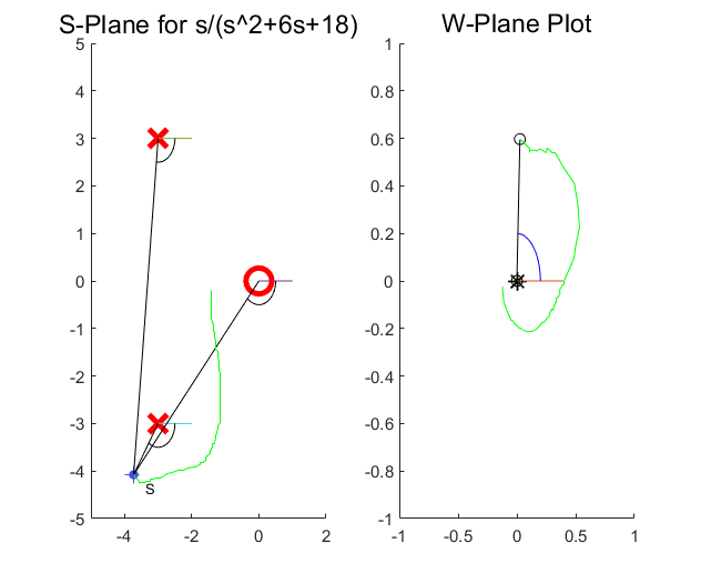
1. S平面和W平面：

   • 该程序展示了两个子图：左边是S平面，右边是W平面。S平面中展示了函数$s/(s^2+6s+18)$的极点和零点，W平面则展示了通过该函数映射后的结果。

2. 交互功能：

   • 用户可以通过点击S平面中的点，动态调整该点的坐标，从而改变映射后的W平面中的点位置。程序会自动更新函数值并绘制出相应的轨迹和相位。

3. 动态绘制相位和映射轨迹：

   • 代码使用animatedline实现了动态绘制函数映射的过程，实时更新相位和映射点的位置。DrawPhasor函数用于绘制复数的相位和向量。

4. Cauchy辐角定理的应用：

   • 柯西辐角定理说明，复函数在闭合路径上围绕零点的次数与路径的积分结果有关。该可视化演示了这一原理如何通过图形体现。

代码实现：

function Interact(Pos)
% -------------------------------------------------
%
% A small interative demonstration of Cauchy Argument Principle
% Based on File by Brian Douglas, 
% Updated by Gavin Kane
%   R2015 R2016 Matlab supported with animatedline function replacing
%   delete calls
%   Tracer added to show mapping function
%
% -------------------------------------------------

persistent h1 h2 h3 p0 p1 w1 a1 a2 a3 t0 t1

if nargin == 0
    close all;
    clc;

    hfig = figure();

    subplot(1, 2, 2);
    title('W-Plane Plot', 'Interpreter', 'None', 'FontSize', 14);
    hold on
    plot(0, 0, '*k', 'MarkerSize', 10, 'LineWidth', 1);
    axis([-1 1 -1 1])
    plot([0 .4], [0 0]);

    subplot(1, 2, 1);
    title('S-Plane for s/(s^2+6s+18)', 'Interpreter', 'None', 'FontSize', 14);
    hold on;
    axis([-5 2 -5 5])
    plot(0, 0, 'or', 'MarkerSize', 14, 'LineWidth', 3);
    plot(-3, 3, 'xr', 'MarkerSize', 14, 'LineWidth', 3);
    plot(-3, -3, 'xr', 'MarkerSize', 14, 'LineWidth', 3);

    plot([0 1], [0 0]);
    plot([-3 -2], [3 3]);
    plot([-3 -2], [-3 -3]);
    
    p0 = impoint(gca,-2,0);
    setString(p0,'S');

    h1 = animatedline;
    h2 = animatedline;
    h3 = animatedline;
    a1 = animatedline;
    a2 = animatedline;
    a3 = animatedline;
    t0 = animatedline('color', 'green');
    
    s = -2 + 0*1i;
    val = s/(s^2+6*s+18);
    subplot(1, 2, 2);
    p1 = animatedline('marker', 'o');
    addpoints(p1, [0 real(val)], [0 imag(val)])
    theta5 = atan2(imag(val), real(val));

    if theta5 < 0, theta5 = theta5 + 2*pi; end
    points5 = linspace(0,theta5);
    xCurve5 = (1/5).*cos(points5);  
    yCurve5 = (1/5).*sin(points5); 
    w1 = animatedline('color','blue');
    addpoints(w1, xCurve5, yCurve5)

    t1 = animatedline('color', 'green');

    DrawPhasor(p0, h1, h2, h3, a1, a2, a3, t0)
    
    addNewPositionCallback(p0,@Interact);
    
else

    clearpoints(p1)
    clearpoints(w1)
    s = Pos(1) + Pos(2)*1i;
    val = s/(s^2+6*s+18);
    subplot(1, 2, 2);
    addpoints(p1, [0 real(val)], [0 imag(val)])
    theta5 = atan2(imag(val), real(val));
    if theta5 < 0, theta5 = theta5 + 2*pi; end
    points5 = linspace(0,theta5);
    xCurve5 = (1/5).*cos(points5);  
    yCurve5 = (1/5).*sin(points5); 
    addpoints(w1, xCurve5, yCurve5)
    [x,y] = getpoints(t1);
    if length(x) > 100
        x = x(2:end);
        y = y(2:end);
    end
    clearpoints(t1)
    addpoints(t1, [x real(val)], [y imag(val)])
    
    DrawPhasor(p0, h1, h2, h3, a1, a2, a3, t0)
    
end
end

function DrawPhasor(p0, h1, h2, h3, a1, a2, a3, t0, t1)

    P = zeros(1,2);
    P(1,:) = getPosition(p0);
    subplot(1, 2, 1);

    clearpoints(h1)
    clearpoints(h2)
    clearpoints(h3)
    clearpoints(a1)
    clearpoints(a2)
    clearpoints(a3)
    
    addpoints(h1, [0 P(:,1)], [0, P(:,2)]);
    addpoints(h2, [-3 P(:,1)], [3, P(:,2)]);
    addpoints(h3, [-3 P(:,1)], [-3, P(:,2)]);
    
    theta1 = atan2(P(:,2), P(:,1));
    points1 = linspace(0,theta1);
    xCurve1 = (1/2).*cos(points1);  
    yCurve1 = (1/2).*sin(points1); 
    addpoints(a1, xCurve1, yCurve1);
    
    theta2 = atan2(P(:,2) +  3, P(:,1) + 3);
    points2 = linspace(0,theta2);
    xCurve2 = -3 + (1/2).*cos(points2);  
    yCurve2 = -3 + (1/2).*sin(points2); 
    addpoints(a2, xCurve2, yCurve2);
    
    theta3 = atan2(P(:,2) - 3, P(:,1) + 3);
    points3 = linspace(0,theta3);
    xCurve3 = -3 + (1/2).*cos(points3);  
    yCurve3 =  3 + (1/2).*sin(points3); 
    addpoints(a3, xCurve3, yCurve3);
    
    [x,y] = getpoints(t0);
    if length(x) > 100
        x = x(2:end);
        y = y(2:end);
    end
    clearpoints(t0)
    addpoints(t0, [x P(1)], [y P(2)])

end

可视化示例：