基于动态自适应加权极限RUL 预测（Matlab代码实现）

💥💥💞💞欢迎来到本博客❤️❤️💥💥

​

🏆博主优势：🌞🌞🌞博客内容尽量做到思维缜密，逻辑清晰，为了方便读者。

⛳️座右铭：行百里者，半于九十。

目录

💥1 概述

📚2 运行结果

🎉3 参考文献

🌈4 Matlab代码实现

💥1 概述

本文引入了 [1] 中提出的 LCI-ELM 的新改进。创新点侧重于训练模型对更高维度“时变”数据的适应。使用C-MAPSS数据集[2]对所提出的算法进行了研究。PSO[3]和R-ELM[4]训练规则被整合在一起，用于此任务。

[1] Y. X. Wu, D. Liu, and H. Jiang, “Length-Changeable Incremental Extreme Learning Machine,” J. Comput. Sci. Technol., vol. 32, no. 3, pp. 630–643, 2017.
[2] A. Saxena, M. Ieee, K. Goebel, D. Simon, and N. Eklund, “Damage Propagation Modeling for Aircraft Engine Prognostics,” Response, 2008.
[3] M. N. Alam, “Codes in MATLAB for Particle Swarm Optimization Codes in MATLAB for Particle Swarm Optimization,” no. March, 2016.
[4] J. Cao, K. Zhang, M. Luo, C. Yin, and X. Lai, “Extreme learning machine and adaptive sparse representation for image classification,” Neural Networks, vol. 81, no. 61773019, pp. 91–102, 2016.

📚2 运行结果

部分代码：

%% Options 
Options.k=10;                     % incremental lraning parameters
Options.lambda=0.7;               % incremental lraning parameters
Options.MaxHiddenNeurons=100;     % maximaum number of hidden neurons
Options.ActivationFunType='radbas';  % activation function
population=exp(-0:0.5:4)';        % generate random initial population
Options.C(:,1)=population;        % regularization parameter
Options.Weighted=population;      % weighted ELM parameters
Options.epsilon=1e-3;             % desired tolerance error
%% PSO
Options.epsilonPSO=10e-3; % desired tolerance error
Options.LB=100;           % Lower bounds constraints
Options.UB=-100;          % Upper bounds constraints
Options.maxite=3;         % maximum number of iterations
Options.wmax=0.2;         % inertial weight
Options.wmin=0.2;         % inertial weight
Options.c1=2;             % acceleration factor
Options.c2=2;             % acceleration factor
%% dataset
load('FD001')
xtr=DATA.X_batch;
ytr=DATA.Y_batch;
xts=DATA.Xts_batch;
yts=DATA.Yts_batch;
%% Training
i=17;
[neta] = LCIELM(xtr,ytr,xts,yts,DATA.Xts{i},Options)        % LCI-ELM
[netb] = LOO_RT_LCI_ELM(xtr,ytr,xts,yts,DATA.Xts{i},Options)% Leave One Out Regularized LCI-ELM
[netc] = OP_W_LCI_ELM(xtr,ytr,xts,yts,DATA.Xts{i},Options)  % PSO for weighted LCI-ELM
%% Plot population variation 
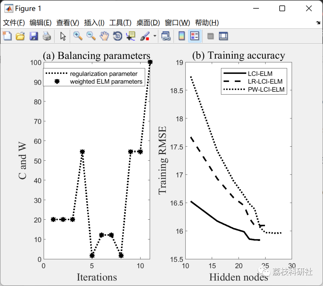
subplot(121)
plot(1:length(netc.reg(:,2)),netc.reg(:,2),'k:'...
     ,1:length(netc.reg(:,2)),netc.reg(:,1),'k*'...
     ,'LineWidth',2)
xlabel('Iterations'...
 ,'FontName','Times New Roman','FontSize',14)
ylabel('C and W'...
 ,'FontName','Times New Roman','FontSize',14)
title('(a) Balancing parameters'...
 ,'FontName','Times New Roman','FontSize',14) 
legend('regularization parameter','weighted ELM parameters')
%% plot (Error)
subplot(122)

f=30;
plot(neta.nodes,smooth(neta.E,f),'k',...
    netb.nodes,smooth(netb.E,f),'k--',...
    netc.nodes,smooth(netc.E,f),...
   'k:','LineWidth',2);
xlabel('Hidden nodes'...
 ,'FontName','Times New Roman','FontSize',14)
ylabel('Training RMSE'...
 ,'FontName','Times New Roman','FontSize',14)
title('(b) Training accuracy'...
 ,'FontName','Times New Roman','FontSize',14)
legend('LCI-ELM','LR-LCI-ELM','PW-LCI-ELM');

%% plot (Score)
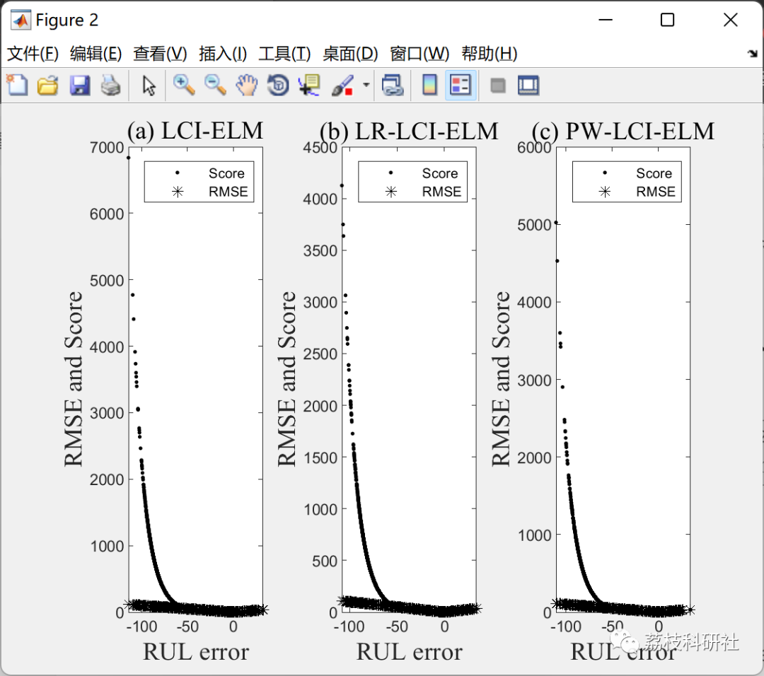
figure(2)
subplot(131)
plot(neta.d,neta.S,'k.',neta.d,neta.er,'k*')
xlabel('RUL error'...
 ,'FontName','Times New Roman','FontSize',14)
ylabel('RMSE and Score'...
 ,'FontName','Times New Roman','FontSize',14)
title('(a) LCI-ELM'...
 ,'FontName','Times New Roman','FontSize',14)
legend('Score','RMSE');
%%%%
subplot(132)
plot(netb.d,netb.S,'k.',netb.d,netb.er,'k*')
xlabel('RUL error'...
 ,'FontName','Times New Roman','FontSize',14)
ylabel('RMSE and Score'...
 ,'FontName','Times New Roman','FontSize',14)
title('(b) LR-LCI-ELM'...
 ,'FontName','Times New Roman','FontSize',14)
legend('Score','RMSE');
%%%%
subplot(1,3,3)
plot(netc.d,netc.S,'k.',netc.d,netc.er,'k*')
xlabel('RUL error'...
 ,'FontName','Times New Roman','FontSize',14)
ylabel('RMSE and Score'...
 ,'FontName','Times New Roman','FontSize',14)
title('(c) PW-LCI-ELM'...
 ,'FontName','Times New Roman','FontSize',14)
legend('Score','RMSE');
%%%%

🎉3 参考文献

[1] Y. X. Wu, D. Liu, and H. Jiang, “Length-Changeable Incremental Extreme Learning Machine,” J. Comput. Sci. Technol., vol. 32, no. 3, pp. 630–643, 2017.
[2] A. Saxena, M. Ieee, K. Goebel, D. Simon, and N. Eklund, “Damage Propagation Modeling for Aircraft Engine Prognostics,” Response, 2008.
[3] M. N. Alam, “Codes in MATLAB for Particle Swarm Optimization Codes in MATLAB for Particle Swarm Optimization,” no. March, 2016.
[4] J. Cao, K. Zhang, M. Luo, C. Yin, and X. Lai, “Extreme learning machine and adaptive sparse representation for image classification,” Neural Networks, vol. 81, no. 61773019, pp. 91–102, 2016.

🌈4 Matlab代码实现