用于计算方差敏感索波尔指数方法，这是一种流行的特征选择和降维算法（Matlab代码实现）

 💥💥💞💞欢迎来到本博客❤️❤️💥💥

🏆博主优势：🌞🌞🌞博客内容尽量做到思维缜密，逻辑清晰，为了方便读者。

⛳️座右铭：行百里者，半于九十。

📋📋📋本文目录如下：🎁🎁🎁

目录

💥1 概述

📚2 运行结果

🎉3 参考文献

🌈4 Matlab代码实现

---

💥1 概述

方差敏感索波尔指数（Variance Sensitive ReliefF，VS-ReliefF）是一种用于特征选择和降维的流行算法，它基于ReliefF算法进行改进。ReliefF算法是一种经典的特征选择算法，通过对特征之间的距离进行估计，找到对目标属性有区分度的特征。

VS-ReliefF算法与ReliefF算法的主要区别在于，在进行特征权重估计时，VS-ReliefF算法考虑了特征之间的方差信息，以增强对非线性关系的适应能力。这使得VS-ReliefF算法在处理数据中存在方差敏感特征的情况下表现更好，能够更准确地进行特征选择和降维。

总的来说，VS-ReliefF算法通过综合考虑特征之间的距离和方差信息，提高了特征选择和降维的性能，适用于处理具有复杂数据特征关系的情况。

📚2 运行结果

算例：

主函数代码：

%% Assume uncorrelated inputs
% the samples
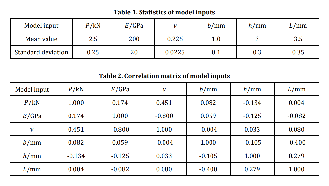
Mu = [2.5,200,0.225,1.0,3,3.5]; % mean value
Std = Mu*0.1; % standard deviation
Sigma = diag(Std.^2); % standard deviation;
N = 2e5;
n = 2e3;
input_sample = lhsnorm(Mu, Sigma, N);

% the double loop method
First_order_double_loop   = GSA_FirstOrder(input_sample, @func_beam, n);
Total_effects_double_loop = GSA_TotalEffect(input_sample, @func_beam, n);

% Saltelli's single loop method
A = input_sample;
B = lhsnorm(Mu, Sigma, N);
First_order_Saltelli = Sen_FirstOrder_Saltelli(A, B, @func_beam);
Total_effects_Saltelli = Sen_TotalEffect_Saltelli(A, B, @func_beam);

% Sobol' method
First_order_Sobol = Sen_FirstOrder_Sobol_07(A, B, @func_beam);

% improved FAST based on RBD
k = size(Mu, 2);
First_order_FAST = Sen_FirstOrder_RBD(N, k, @beam_RBD, Mu, Std);

%% plot
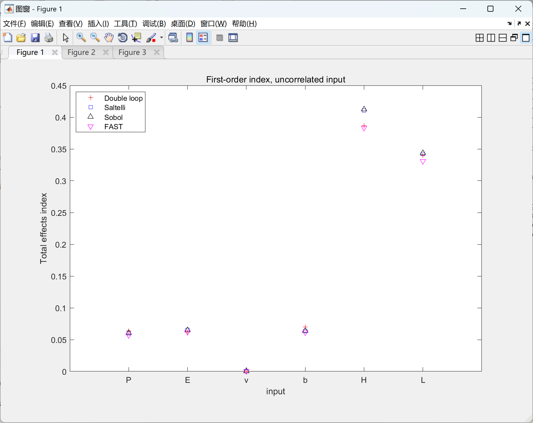
figure(1)
plot(First_order_double_loop, 'r+'); hold on;
plot(First_order_Saltelli, 'bs'); hold on;
plot(First_order_Sobol, 'k^'); hold on;
plot(First_order_FAST, 'mv');
xlim([0, 7]);
set(gca, 'XTickLabel',{'P','E','v','b','H','L'},'XTick',[1 2 3 4 5 6]);
xlabel('input')
ylabel('Total effects index')
legend({'Double loop', 'Saltelli', 'Sobol', 'FAST'}, 'location', 'northwest')
title('First-order index, uncorrelated input')

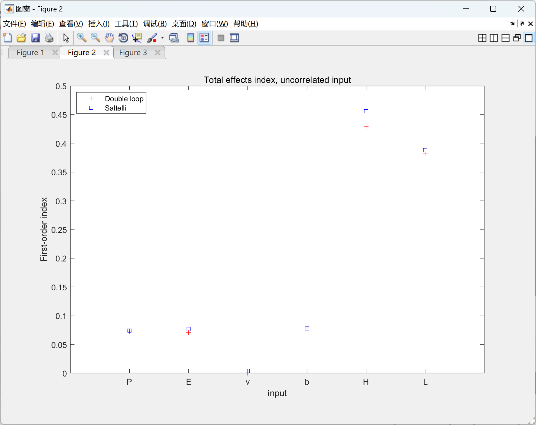
figure(2)
plot(Total_effects_double_loop, 'r+'); hold on;
plot(Total_effects_Saltelli, 'bs'); hold on;
xlim([0, 7]);
set(gca, 'XTickLabel',{'P','E','v','b','H','L'},'XTick',[1 2 3 4 5 6]);
xlabel('input')
ylabel('First-order index')
legend({'Double loop', 'Saltelli'}, 'location', 'northwest')
title('Total effects index, uncorrelated input')

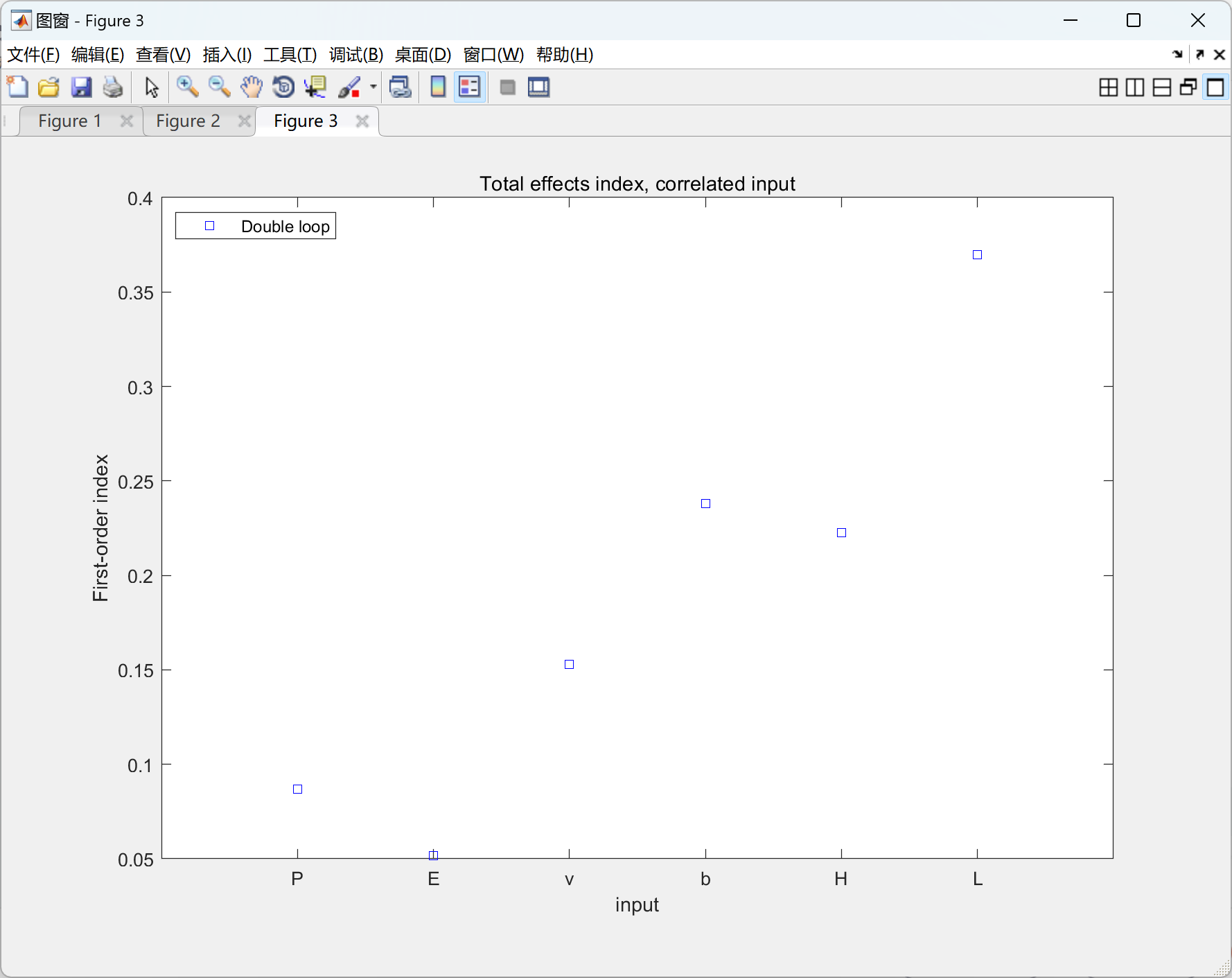
%% Assume correlated inputs
corr = [1    0.174    0.451    0.082    -0.134    0.004;
0.174    1    -0.8    0.059    -0.125    -0.082;
0.451    -0.8    1    -0.004    0.033    0.08;
0.082    0.059    -0.004    1    -0.105    -0.4;
-0.134    -0.125    0.033    -0.105    1    0.279;
0.004    -0.082    0.08    -0.4    0.279    1]; % correlation matrix

COV = zeros(k, k);
for i = 1:k
    for j = 1:k
        COV(i, j) = corr(i, j) * Std(i) * Std(j);
    end
end
First_order_double_loop_2 = GSA_FirstOrder_mvn(Mu', COV, @func_beam, 1000);

figure(3)
plot(First_order_double_loop_2, 'bs'); hold on;
xlim([0, 7]);
set(gca, 'XTickLabel',{'P','E','v','b','H','L'},'XTick',[1 2 3 4 5 6]);
xlabel('input')
ylabel('First-order index')
legend({'Double loop'}, 'location', 'northwest')
title('Total effects index, correlated input')
 

🎉3 参考文献

文章中一些内容引自网络，会注明出处或引用为参考文献，难免有未尽之处，如有不妥，请随时联系删除。

[1]员婉莹,吕震宙,牟珊珊.一种高效计算各类基于方差灵敏度指标的方法[J].北京航空航天大学学报, 2016(4):10.DOI:10.13700/j.bh.1001-5965.2015.0309.

[2]徐忠明.模型互相关参数敏感性分析方法及其应用研究[J].[2024-03-21].

🌈4 Matlab代码实现