深入理解R包AUcell对于分析单细胞的作用

首先我们来看看对AUcell的介绍
AUCell可以识别单细胞RNA序列数据中具有活跃基因集（例如signatures，基因模块...）的细胞。 AUCell使用“曲线下面积”（AUC）来计算输入基因集的关键子集是否在每个细胞的表达基因中富集。 AUC分数在所有细胞中的分布允许探索特征的相对表达。 由于计分方法是基于排名的，因此AUCell不受基因表达单位和标准化程序的影响。 此外，由于对cell进行了单独评估，因此可以轻松地将其应用于更大的数据集，并根据需要对表达式矩阵进行分组。
那也就是说，AUcell是分析感兴趣的基因集在所有细胞是否存在富集，道理很简单，我们来看看主要分析内容
用AUcell进行分析分三步：
1、 Build the rankings
2、Calculate the Area Under the Curve (AUC)
3、Set the assignment thresholds

我们首先来分析第一步：AUcell首先是对cell怎么排序的。

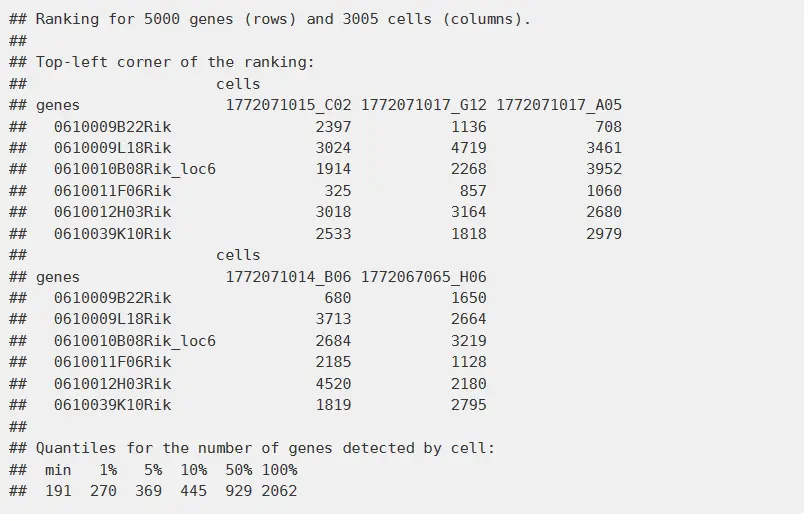
For each cell, the genes are ranked from highest to lowest value. The genes with same expression value are shuffled. Therefore, genes with expression ‘0’ are randomly sorted at the end of the ranking. It is important to check that most cells have at least the number of expressed/detected genes that are going to be used to calculate the AUC (aucMaxRank in calcAUC()). The histogram provided by AUCell_buildRankings() allows to quickly check this distribution. plotGeneCount(exprMatrix) allows to obtain only the plot before building the rankings.
这个地方我们可以看出，对于每个基因，从高到底进行排名，也就是说每个细胞的每个基因都有一个排名，得到一个排名的矩阵。

接下来第二步：

1. Calculate enrichment for the gene signatures (AUC)
   首先我们要知道什么是AUC曲线：
   AUC（Area Under Curve）被定义为ROC下与坐标轴围成的面积，显然这个面积的数值不会大于1。又由于ROC曲线一般都处于y=x这条直线的上方，所以AUC的取值范围在0.5和1之间。AUC越接近1.0，检测方法真实性越高;等于0.5时，则真实性最低，无应用价值。
   那么什么是ROC曲线呢？
   一、 ROC曲线的由来
   很多学习器是为测试样本产生一个实值或概率预测，然后将这个预测值与一个分类阈值进行比较，若大于阈值则分为正类，否则为反类。例如，神经网络在一般情形下是对每个测试样本预测出一个[0.0，1.0]之间的实值，然后将这个值与阈值0.5进行比较，大于0.5则判为正例，否则为反例。这个阈值设置的好坏，直接决定了学习器的泛化能力。
   在不同的应用任务中，我们可根据任务需求来采用不同的阈值。例如，若我们更重视“查准率”，则可以把阈值设置的大一些，让分类器的预测结果更有把握；若我们更重视“查全率”，则可以把阈值设置的小一些，让分类器预测出更多的正例。因此，阈值设置的好坏，体现了综合考虑学习器在不同任务下的泛化性能的好坏。为了形象的描述这一变化，在此引入ROC曲线，ROC曲线则是从阈值选取角度出发来研究学习器泛化性能的有力工具。
   如果你还对“查准率”和“查全率”不了解，看我之前的文章【错误率、精度、查准率、查全率和F1度量】详细介绍

二、 什么是ROC曲线

ROC全称是“受试者工作特征”(Receiver OperatingCharacteristic)曲线。我们根据学习器的预测结果，把阈值从0变到最大，即刚开始是把每个样本作为正例进行预测，随着阈值的增大，学习器预测正样例数越来越少，直到最后没有一个样本是正样例。在这一过程中，每次计算出两个重要量的值，分别以它们为横、纵坐标作图，就得到了“ROC曲线”。

** ROC曲线的纵轴是“真正例率”(True Positive Rate, 简称TPR)，横轴是“假正例率”(False Positive Rate,简称FPR)，**基于上篇文章《错误率、精度、查准率、查全率和F1度量》的表1中符号，两者分别定义为：

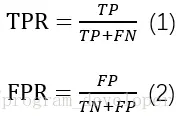
image

显示ROC曲线的图称为“ROC图”。图1给出了一个示意图，显然，对角线对应于“随机猜测”模型，而点(0,1)则对应于将所有正例预测为真正例、所有反例预测为真反例的“理想模型”。

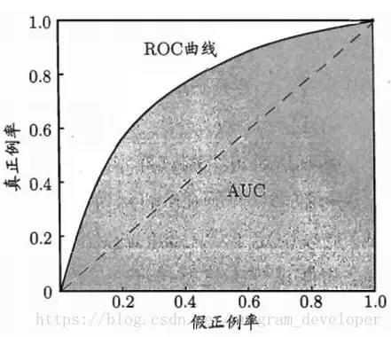
图1：ROC曲线与AUC面积

现实任务中通常是利用有限个测试样例来绘制ROC图，此时仅能获得有限个(真正例率，假正例率)坐标对，无法产生图1中的光滑ROC曲线，只能绘制出图2所示的近似ROC曲线。绘制过程很简单：给定m+ 个正例和m-个反例，根据学习器预测结果对样例进行排序，然后把分类阈值设置为最大，即把所有样例均预测为反例，此时真正例率和假正例率均为0，在坐标(0,0)处标记一个点。然后，将分类阈值依次设为每个样例的预测值，即依次将每个样例划分为正例。设前一个标记点坐标为

，当前若为真正例，则对应标记点的坐标为

；当前若为假正例，则对应标记点的坐标为

，然后用线段连接相邻点即得。

三、 ROC曲线的意义

（1）主要作用

1. ROC曲线能很容易的查出任意阈值对学习器的泛化性能影响。

2.有助于选择最佳的阈值。ROC曲线越靠近左上角，模型的查全率就越高。最靠近左上角的ROC曲线上的点是分类错误最少的最好阈值，其假正例和假反例总数最少。

3.可以对不同的学习器比较性能。将各个学习器的ROC曲线绘制到同一坐标中，直观地鉴别优劣，靠近左上角的ROC曲所代表的学习器准确性最高。

（2）优点

1. 该方法简单、直观、通过图示可观察分析方法的准确性，并可用肉眼作出判断。ROC曲线将真正例率和假正例率以图示方法结合在一起，可准确反映某种学习器真正例率和假正例率的关系，是检测准确性的综合代表。

2. 在生物信息学上的优点：ROC曲线不固定阈值，允许中间状态的存在，利于使用者结合专业知识，权衡漏诊与误诊的影响，选择一个更加的阈值作为诊断参考值。

四、 AUC面积的由来

如果两条ROC曲线没有相交，我们可以根据哪条曲线最靠近左上角哪条曲线代表的学习器性能就最好。但是，实际任务中，情况很复杂，如果两条ROC曲线发生了交叉，则很难一般性地断言谁优谁劣。在很多实际应用中，我们往往希望把学习器性能分出个高低来。在此引入AUC面积。

在进行学习器的比较时，若一个学习器的ROC曲线被另一个学习器的曲线完全“包住”，则可断言后者的性能优于前者；若两个学习器的ROC曲线发生交叉，则难以一般性的断言两者孰优孰劣。此时如果一定要进行比较，则比较合理的判断依据是比较ROC曲线下的面积，即AUC(Area Under ROC Curve)，如图1图2所示。

五、 什么是AUC面积

** AUC就是ROC曲线下的面积，衡量学习器优劣的一种性能指标。**从定义可知，AUC可通过对ROC曲线下各部分的面积求和而得。假定ROC曲线是由坐标为

的点按序连接而形成，参见图2，则AUC可估算为公式3。

六、 AUC面积的意义

AUC是衡量二分类模型优劣的一种评价指标，表示预测的正例排在负例前面的概率。

看到这里，是不是很疑惑，根据AUC定义和计算方法，怎么和预测的正例排在负例前面的概率扯上联系呢？如果从定义和计算方法来理解AUC的含义，比较困难，实际上AUC和Mann-WhitneyU test(曼-慧特尼U检验)有密切的联系。从Mann-Whitney U statistic的角度来解释，AUC就是从所有正样本中随机选择一个样本，从所有负样本中随机选择一个样本，然后根据你的学习器对两个随机样本进行预测，把正样本预测为正例的概率p1，把负样本预测为正例的概率p2,p1 > p2的概率就等于AUC。所以AUC反映的是分类器对样本的排序能力。根据这个解释，如果我们完全随机的对样本分类，那么AUC应该接近0.5。
另外值得注意的是，AUC的计算方法同时考虑了学习器对于正例和负例的分类能力，在样本不平衡的情况下，依然能够对分类器做出合理的评价。AUC对样本类别是否均衡并不敏感，这也是不均衡样本通常用AUC评价学习器性能的一个原因。例如在癌症预测的场景中，假设没有患癌症的样本为正例，患癌症样本为负例，负例占比很少(大概0.1%)，如果使用准确率评估，把所有的样本预测为正例便可以获得99.9%的准确率。但是如果使用AUC，把所有样本预测为正例，TPR为1，FPR为1。这种情况下学习器的AUC值将等于0.5，成功规避了样本不均衡带来的问题。
最后，我们在讨论一下：在多分类问题下能不能使用ROC曲线来衡量模型性能？
我的理解：ROC曲线用在多分类中是没有意义的。只有在二分类中Positive和Negative同等重要时候，适合用ROC曲线评价。如果确实需要在多分类问题中用ROC曲线的话，可以转化为多个“一对多”的问题。即把其中一个当作正例，其余当作负例来看待，画出多个ROC曲线。

回到我们生信分析的第二步，对于AUC的计算
To determine whether the gene set is enriched at the top of the gene-ranking for each cell, AUCell uses the “Area Under the Curve” (AUC) of the recovery curve.
In order to calculate the AUC, by default only the top 5% of the genes in the ranking are used (i.e. checks whether the genes in the gene-set or signature are within the top 5%). This allows faster execution on bigger datasets, and reduce the effect of the noise at the bottom of the ranking (e.g. where many genes might be tied at 0 counts). The percentage to take into account can be modified with the argument aucMaxRank. For datasets where most cells express many genes (e.g. a filtered dataset), or these have high expression values, it might be good to increase this threshold. Check the histogram provided by AUCell_buildRankings to get an estimation on where this threshold lies within the dataset.
这里我们深入理解一下，对于一个细胞进行基因排序之后，得到下面的图：

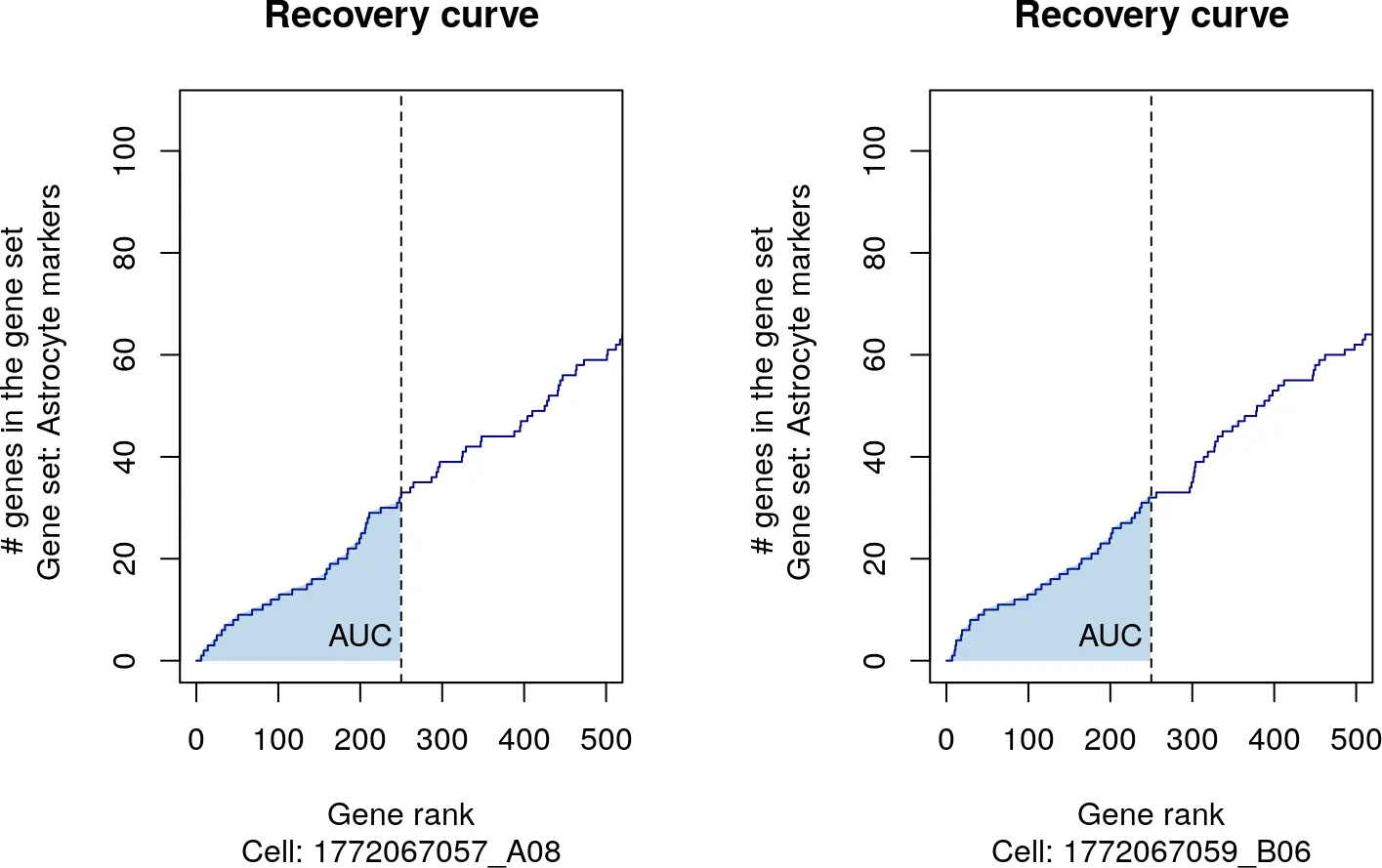
也就是说，看看排名前250位的基因在排名慢慢变大的过程中，包含基因集数量的变化，而形成了一条曲线，曲线下面的面积，就是我们得到的富集分数。（似乎和刚才讲的ROC没什么关系~~）
The AUC estimates the proportion of genes in the gene-set that are highly expressed in each cell. Cells expressing many genes from the gene-set will have higher AUC values than cells expressing fewer (i.e. compensating for housekeeping genes, or genes that are highly expressed in all the cells in the dataset). Since the AUC represents the proportion of expressed genes in the signature, we can use the relative AUCs across the cells to explore the population of cells that are present in the dataset according to the expression of the gene-set.
However, determining whether the signature is active (or not) in a given cell is not always trivial. The AUC is not an absolute value, but it depends on the the cell type (i.e. sell size, amount of transcripts), the specific dataset (i.e. sensitivity of the measures) and the gene-set. It is often not straight forward to obtain a pruned signature of clear marker genes that are completely “on” in the cell type of interest and off" in every other cell. In addition, at single-cell level, most genes are not expressed or detected at a constant level.
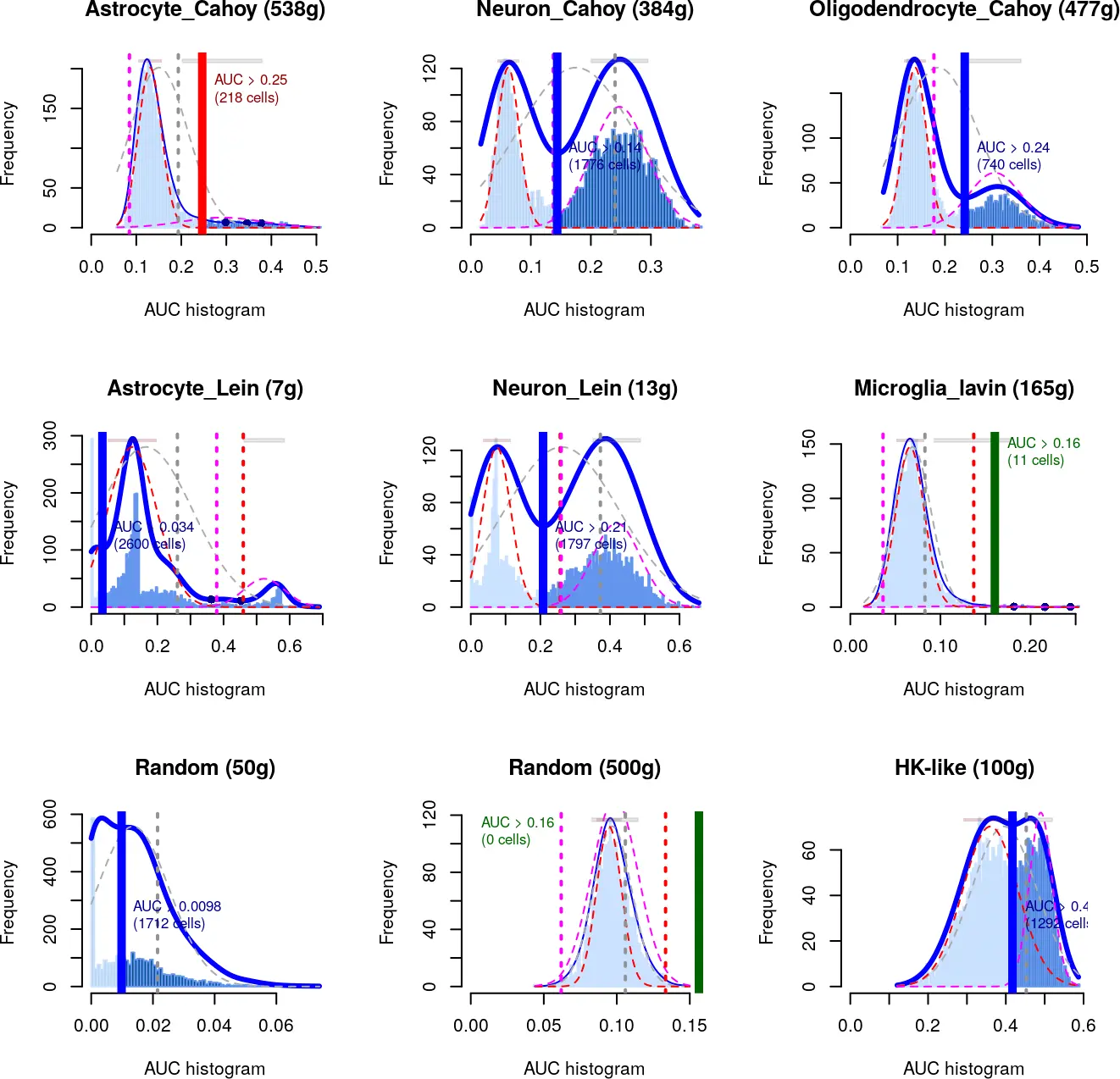
The ideal situation will be a bi-modal distribution, in which most cells in the dataset have a low “AUC” compared to a population of cells with a clearly higher value (i.e. see “Oligodendrocites” in the next figure). This is normally the case on gene sets that are active mostly in a population of cells with a good representation in the dataset (e.g. ~ 5-30% of cells in the dataset). Similar cases of “marker” gene sets but with different proportions of cells in the datasets are the “neurons” and “microglia” (see figure). When there are very few cells within the dataset, the distribution might look normal-like, but with some outliers to the higher end (e.g. microglia). While if the gene set is marker of a high percentage of cells in the dataset (i.e. neurons), the distribution might start approaching the look of a gene-set of housekeeping genes. As example, the ‘housekeeping’ gene-set in the figure includes genes that are detected in most cells in the dataset.
Note that the size of the gene-set will also affect the results. With smaller gene-genes (fewer genes), it is more likely to get cells with AUC = 0. While this is the case of the “perfect markers” it is also easier to get it by chance with smal datasets. (i.e. Random gene set with 50 genes in the figure). Bigger gene-sets (100-2k) can be more stable and easier to evaluate, as big random gene sets will approach the normal distibution.
To ease the exploration of the distributions, the function AUCell_exploreThresholds() automatically plots all the histograms and calculates several thresholds that could be used to consider a gene-set ‘active’ (returned in aucThr). The distributions are plotted as dotted lines over the histogram and the corresponding thresholds as vertical bars in the matching color. The thicker vertical line indicates the threshold selected by default (aucThr selected): the highest value to reduce the false positives.

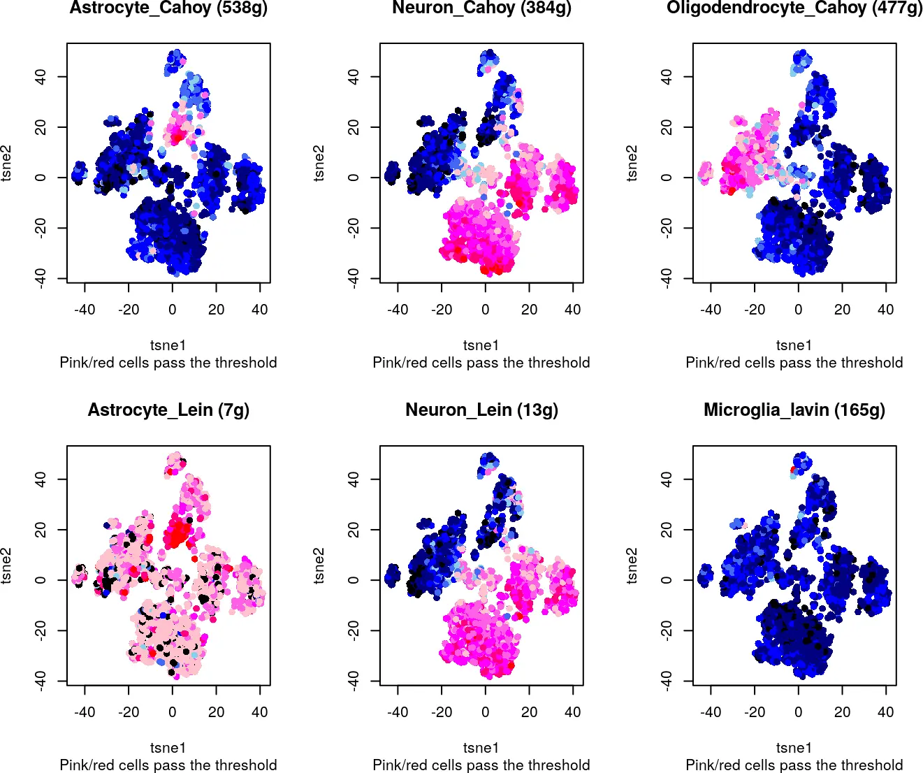
而将具有较高AUC值反映到细胞中，可以得到

至于代码很简单：

library(AUCell)
cells_rankings <- AUCell_buildRankings(exprMatrix)##基因排序
cells_AUC <- AUCell_calcAUC(geneSets, cells_rankings, aucMaxRank=nrow(cells_rankings)*0.05) ##计算AUC值。
cells_assignment <- AUCell_exploreThresholds(cells_AUC, plotHist=TRUE, nCores=1,assign=TRUE)##挑选阈值

至于基因集的选择，可以借助于hallmark，用于研究肿瘤特征分析。