[slam]点云帧间匹配

六树蚊

已于 2024-02-01 13:22:49 修改

阅读量1.3k

点赞数 24

文章标签：算法人工智能

于 2024-01-23 14:05:29 首次发布

本文链接：https://blog.csdn.net/weixin_55533898/article/details/135769725

版权

一. 基本原理

通过两帧数据的匹配计算两帧间的变换矩阵
设上一帧点云数据集为{pi}，当前点云数据集为{pi’}，求解旋转矩阵R和平移向量t，使得：

$min(E(R,t)) = min(\frac{1}{N}*\sum||p_i-(R*p_i'+t)||^{2})$

二. ICP及其变种

2.1 点到点的匹配

主要有ICP，VICP，NICP算法
ICP：寻找最近点，通过距离最小迭代出变换矩阵
VICP：去除激光畸变后的ICP算法
NICP：距离的基础上，增加法向角度，曲率的限制，剔除错误匹配对后计算变换矩阵

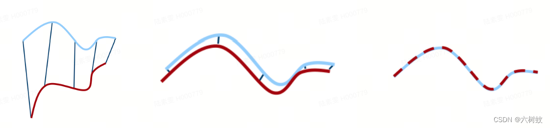
2.2 点到线的匹配

主要有PL_ICP算法
背景：每次激光扫描时，未必会扫描到同一个点，匹配点更有可能在线上
方法：寻找最近的两个点，计算当前点离最近两点形成的直线距离，计算变换矩阵

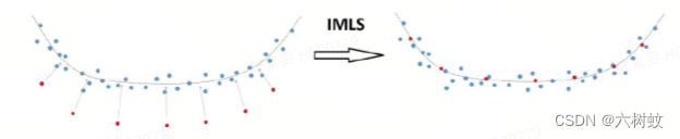
2.3 点到面的匹配

主要有IMLS_ICP算法
背景：每次激光扫描时，未必会扫描到同一个点，也未必会扫描到之前帧激光点构建的子图所在的线段上，但大概率会扫描到之前帧激光点所在的平面上
方法：通过上一帧激光数据重建曲面，找当前激光点在曲面上的投影，组成匹配对，再通过ICP方式找到转换矩阵

2.4 面到面的匹配

主要有GICP算法

三. ICP算法

3.1 ICP的位姿解为

$R = V*U^{t}\\t=p-R*p'$

公式中变量含义：
pi和pi′为两帧点云数据
p,p'为两帧数据的几何中心（均值）
qi和qi′为点云去中心化后数据
V,Ut为qi∗qi′t进行SVD分解得到

R，t为两帧的变换矩阵

3.2 ICP算法的推导过程：

1. 计算点云的几何中心（均值）

$p = \frac{1}{N}*\sum{p_i}$

$p' = \frac{1}{N}*\sum{p_i'}$

2. 去中心化后

$q_i = p_i-p$

$q_i' = p_i'-p'$

3. 求最小二乘

原最小二乘：

$\sum ^{2} = \sum||p_i'-(Rp_i+T)||^{2}$

转换为：

$\sum ^{2} = \sum||q_i'-R*q_i||^{2}=\sum(q_i'-R*q_i)^{t}*(q_i'-R*q_i)\\=\sum(q_i'^{t}*q_i'+q_i^{t}*q_i-2*q_i'^{t}*R*q_i)$

求min $\sum ^{2}$ ，相当于求max（ $\sum q_i'^{t}*R*q_i$ ）

矩阵乘法及 trace 的定义可得：

$\sum q_i'^{t}*R*q_i = trance(q_i'^{t}*R*q_i )$

根据 trace 的性质：

$trance(AB) = trance(BA)$

即求：

$max(trance( R*q_i*q_i'^{t}))$

令 $H = q_i*q_i'^{t}$ ，即求：

$max(trance( R*H))$

据定理，A为正定对称矩阵，对于任意的正交矩阵都有：

$trance (A*A^{t}) \geq trance (B*A*A^{t})$

H并非正定对称矩阵，所以对H进行SVD分解：

$H = U*\Lambda*V^{t}$

其中U和V为正交矩阵，Λ为对角矩阵

令 $X=V*U^{t}$ ，X为正交矩阵，X*H为正定对称矩阵

$X*H = V*U^{t}*U*\Lambda*V^{t}=V*\Lambda*V^{t}$

所以任意的正交矩阵B，都有：

$trace(X*H)\geq trace(B*X*H)$

所以：

$R = X=V*U^{t}\\t=p-R*p'$

3.3 PCL库中的ICP代码应用(c++)

应用：

// 需要安装pcl库
#include <pcl/point_types.h>
#include <pcl/registration/icp.h>
// 处理出上一帧和当前帧的点云数据
pcl::PointCloud<pcl::PointXYZ>::Ptr cloud_source(new pcl::PointCloud<pcl::PointXYZ>);
pcl::PointCloud<pcl::PointXYZ>::Ptr cloud_target(new pcl::PointCloud<pcl::PointXYZ>);
pcl::IterativeClosestPoint<pcl::PointXYZ, pcl::PointXYZ> icp;
icp.setInputSource(cloud_source);
icp.setInputTarget(cloud_target);
pcl::PointCloud<pcl::PointXYZ> Final;
// 点云配准
// 1.KdTree查找对应点对、剔除错误对应点
// 2.计算R和T的变换矩阵
// 3.迭代
icp.align(Final);
std::cout << "transformation: " << std::endl << icp.getFinalTransformation() << std::endl;

PCL库中的ICP核心源码

/// ICP中的核心代码
template <typename PointSource, typename PointTarget, typename Scalar> 
void pcl::registration::TransformationEstimationSVD<PointSource, PointTarget, Scalar>::getTransformationFromCorrelation (
    const Eigen::Matrix<Scalar, Eigen::Dynamic, Eigen::Dynamic> &cloud_src_demean,   // 移除平均值后的点云 
    const Eigen::Matrix<Scalar, 4, 1> &centroid_src,
    const Eigen::Matrix<Scalar, Eigen::Dynamic, Eigen::Dynamic> &cloud_tgt_demean,
    const Eigen::Matrix<Scalar, 4, 1> &centroid_tgt,
    Matrix4 &transformation_matrix) const
{
  transformation_matrix.setIdentity ();

  // Assemble the correlation matrix H = source * target'
  Eigen::Matrix<Scalar, 3, 3> H = (cloud_src_demean * cloud_tgt_demean.transpose ()).topLeftCorner (3, 3);

  // Compute the Singular Value Decomposition
  Eigen::JacobiSVD<Eigen::Matrix<Scalar, 3, 3> > svd (H, Eigen::ComputeFullU | Eigen::ComputeFullV);
  Eigen::Matrix<Scalar, 3, 3> u = svd.matrixU ();
  Eigen::Matrix<Scalar, 3, 3> v = svd.matrixV ();

  // R 最优证明，提取关键点——正交阵可能为旋转阵或者反射阵，区分行列式 1 或 -1，见下述
  // R 为正交标准阵，故旋转阵行列式应为 1，三维同适用（正交阵相乘保持正交），故判断 det(R)，证明前提可用，以保证计算结果正确
  // 理论支撑 1，两个矩阵乘积的行列式与矩阵行列式的乘积相等
  // 理论支撑 2，矩阵的行列式矩阵转置的行列式相等
  // Compute R = V * U'
  if (u.determinant () * v.determinant () < 0)
  {
    // H = UΣV' 中奇异值最小为 0，即共面，故改变 v 第三维而不改变 H = UΣV' 结果，但由反射转换到 R 旋转的假设
    for (int x = 0; x < 3; ++x)
      v (x, 2) *= -1;
    // 理论上还有一种情况，无奇异值为 0，即非共面，SVD 方法失效，需要用其他如 RANSAC-like 方法对抗离群数据过多
  }
  
  // R 最优证明，即多项式（内积非负）负值项最大化。内积转换为迹，用到 Schwarz 不等式，SVD 分解，定义最优 R，得证，无需再旋转
  Eigen::Matrix<Scalar, 3, 3> R = v * u.transpose ();

  // T 计算，旋转后源中心点 - 目标中心点，取其负值，即源点云转换到目标点云
  // Return the correct transformation
  transformation_matrix.topLeftCorner (3, 3) = R;
  const Eigen::Matrix<Scalar, 3, 1> Rc (R * centroid_src.head (3));
  transformation_matrix.block (0, 3, 3, 1) = centroid_tgt.head (3) - Rc;   // 输出的转换矩阵
}

3.4 ICP代码实现(python)

二维可直接用该方法计算, 避免svd分解等矩阵运算, 具体理论推导见参考资料

import numpy as np
import math
import matplotlib.pyplot as plt

# 求出两个点之间的向量弧度，向量方向由点1指向点2
def GetTheAngleOfTwoPoints(x1,y1,x2,y2):
    return math.atan2(y2-y1,x2-x1)

# 求出两个点的距离
def GetDistOfTwoPoints(x1,y1,x2,y2):
    return math.sqrt(math.pow(x2-x1,2) + math.pow(y2-y1,2))

# 在pt_set点集中找到距(p_x，p_y)最近点的id
def GetClosestID(p_x,p_y,pt_set):
    id = 0
    min = 10000000
    for i in range(pt_set.shape[1]):
        dist = GetDistOfTwoPoints(p_x,p_y,pt_set[0][i],pt_set[1][i])
        if dist < min:
            id = i
            min = dist
    return id

# 求两个点集之间的平均点距
def DistOfTwoSet(set1,set2):
    loss = 0;
    for i in range(set1.shape[1]):
        id = GetClosestID(set1[0][i],set1[1][i],set2)
        dist = GetDistOfTwoPoints(set1[0][i],set1[1][i],set2[0][id],set2[1][id])
        loss = loss + dist
    return loss/set1.shape[1]

def ICP(sourcePoints,targetPoints):
    A = targetPoints # A是标准点云
    B = sourcePoints # B是源点云

    iteration_times = 0 # 迭代次数为0
    dist_now = 1 # A,B两点集之间初始化距离
    dist_improve = 1 # A,B两点集之间初始化距离提升
    dist_before = DistOfTwoSet(A,B) # A,B两点集之间距离
    while iteration_times < 10 and dist_improve > 0.001: # 迭代次数小于10 并且 距离提升大于0.001时，继续迭代
        x_mean_target = A[0].mean() # 获得A点云的x坐标轴均值。
        y_mean_target = A[1].mean() # 获得A点云的y坐标轴均值。
        x_mean_source = B[0].mean() # 获得B点云的x坐标轴均值。
        y_mean_source = B[1].mean() # 获得B点云的y坐标轴均值。

        A_ = A - np.array([[x_mean_target],[y_mean_target]]) # 获得A点云的均一化后点云A_
        B_ = B - np.array([[x_mean_target],[y_mean_target]]) # 获得B点云的均一化后点云B_

        w_up = 0 # w_up，表示角度公式中的分母
        w_down = 0 # w_up，表示角度公式中的分子
        for i in range(A_.shape[1]): # 对点云中每个点进行循环
            j = GetClosestID(A_[0][i],A_[1][i],B) # 在B点云中找到距(A_[0][i],A_[1][i])最近点的id
            w_up_i = A_[0][i]*B_[1][j] - A_[1][i]*B_[0][j] # 获得求和公式，分母的一项
            w_down_i = A_[0][i]*B_[0][j] + A_[1][i]*B_[1][j] # 获得求和公式，分子的一项
            w_up = w_up + w_up_i
            w_down = w_down + w_down_i

        TheRadian = math.atan2(w_up,w_down) # 分母与分子之间的角度
        x = x_mean_target - math.cos(TheRadian)*x_mean_source - math.sin(TheRadian)*y_mean_source # x即为x轴偏移量
        y = x_mean_target + math.cos(TheRadian)*x_mean_source - math.sin(TheRadian)*y_mean_source # y即为y轴偏移量
        R = np.array([[math.cos(TheRadian),math.sin(TheRadian)],[-math.sin(TheRadian),math.cos(TheRadian)]]) # 由θ得到旋转矩阵。

        B = np.matmul(R,B) + np.array([x],[y])

        iteration_times = iteration_times + 1 # 迭代次数+1
        dist_now = DistOfTwoSet(A,B) # 变换后两个点云之间的距离
        dist_improve = dist_before - dist_now # 这一次迭代，两个点云之间的距离提升。
        print("迭代第"+str(iteration_times)+"次，损失是"+str(dist_now)+",提升了"+str(dist_improve)) # 打印迭代次数、损失距离、损失提升
        dist_before = dist_now # 将"现在距离"赋值给"以前距离"，开始下一轮迭代循环。

    return B