scipy应用

1. 求解非线性方程组，cos(a) = 1 - d^2 / (2*r^2) ，L = a * r，d = 140，L = 156; 导入参数雅克比矩阵, 再次进行求解。

#导入优化模块和余弦函数
from scipy.optimize import fsolve
from math import cos
#定义函数
def f(x):
    d=140
    l=156
    a,r=x.tolist()
    return [cos(a)-1+d*d/(2*r*r),l-a*r]
res = fsolve(f,[1,1])
#打印
print("a r")
print(res)
print(f(res))

a r
[ 1.5940638  97.86308398]
[4.596323321948148e-14, 2.7682744985213503e-11]

#导入优化模块和余弦函数
from scipy.optimize import fsolve
from math import cos, sin
#定义函数
def f(x):
    d=140
    l=156
    a,r=x.tolist()
    return [cos(a)-1+d*d/(2*r*r),l-a*r]
#定义导函数
def j(x):
    d=140
    l=156
    a,r=x.tolist()
    return[
        [-sin(a),-(d*d)/(r*r*r)],
        [-r,-a]]
#通过fprime将j的参数传递给fsolve()
res = fsolve(f,[1,1],fprime=j)
#打印
print("a r")
print(res)
print(f(res))

a r
[ 1.5940638  97.86308398]
[-1.3322676295501878e-15, -5.400124791776761e-13]

2、用curve_fit()函数对高斯分布进行拟合，xϵ[0,10],高斯分布函数为y=a*np.exp(-(x-b)**2/(2*c**2)) , 其中真实值a=1,b=5,c=2。试对y加入噪声之后进行拟合, 并作图与真实数据进行比较。(参见课件leastsq(),curve_fit()拟合)

import numpy as np
from scipy.optimize import curve_fit
import matplotlib.pyplot as plt
a = 1; b = 5; c = 2
def gauss(x, a, b, c):
    return a * np.exp(-(x-b) ** 2 / (2 * c ** 2))

x = np.linspace(0, 10, 1000)
y = gauss(x, a, b, c) + np.random.rand(1000) / 50
popt, pcov = curve_fit(gauss, x, y)

y2 = gauss(x, popt[0], popt[1], popt[2])

plt.plot(x, y, 'b-')
plt.plot(x, y2, 'r')
plt.show()

​

​

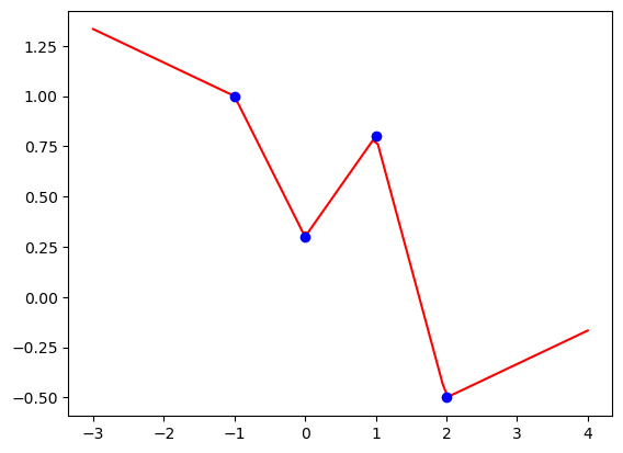
3、对4个数据点x = [-1, 0, 2.0, 1.0]，y = [1.0, 0.3, -0.5, 0.8]进行Rbf插值，插值中使用三种插值方法分别是multiquadric、gaussian、和linear（参见课件5，scipy_rbf.py），需要作点图（加密点）为np.linspace(-3, 4, 100)。

x1 = np.linspace(-3, 4, 100)
y1 = np.linspace(-3, 4, 100)
y1

array([-3.        , -2.92929293, -2.85858586, -2.78787879, -2.71717172,
       -2.64646465, -2.57575758, -2.50505051, -2.43434343, -2.36363636,
       -2.29292929, -2.22222222, -2.15151515, -2.08080808, -2.01010101,
       -1.93939394, -1.86868687, -1.7979798 , -1.72727273, -1.65656566,
       -1.58585859, -1.51515152, -1.44444444, -1.37373737, -1.3030303 ,
       -1.23232323, -1.16161616, -1.09090909, -1.02020202, -0.94949495,
       -0.87878788, -0.80808081, -0.73737374, -0.66666667, -0.5959596 ,
       -0.52525253, -0.45454545, -0.38383838, -0.31313131, -0.24242424,
       -0.17171717, -0.1010101 , -0.03030303,  0.04040404,  0.11111111,
        0.18181818,  0.25252525,  0.32323232,  0.39393939,  0.46464646,
        0.53535354,  0.60606061,  0.67676768,  0.74747475,  0.81818182,
        0.88888889,  0.95959596,  1.03030303,  1.1010101 ,  1.17171717,
        1.24242424,  1.31313131,  1.38383838,  1.45454545,  1.52525253,
        1.5959596 ,  1.66666667,  1.73737374,  1.80808081,  1.87878788,
        1.94949495,  2.02020202,  2.09090909,  2.16161616,  2.23232323,
        2.3030303 ,  2.37373737,  2.44444444,  2.51515152,  2.58585859,
        2.65656566,  2.72727273,  2.7979798 ,  2.86868687,  2.93939394,
        3.01010101,  3.08080808,  3.15151515,  3.22222222,  3.29292929,
        3.36363636,  3.43434343,  3.50505051,  3.57575758,  3.64646465,
        3.71717172,  3.78787879,  3.85858586,  3.92929293,  4.        ])

from scipy.interpolate import Rbf
import numpy as np
import matplotlib.pyplot as plt
x = [-1, 0, 2.0, 1.0]
y = [1.0, 0.3, -0.5, 0.8]
func = Rbf(x, y, function='linear')  # 插值
x1 = np.linspace(-3, 4, 100)
y1 = np.linspace(-3, 4, 100)
z_new = func(x1)
plt.plot(x1, z_new, 'r')
plt.plot(x, y, 'bo')

[<matplotlib.lines.Line2D at 0x1c49bd4cd90>]

​

​

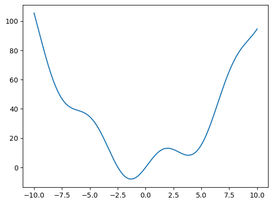
4.分别用optimize.fmin_bfgs、optimize.fminbound、optimize.brute三种优化方法对函数x**2 + 10 * np.sin(x)求最小值，并作图。xϵ[-10, 10].

from scipy.optimize import fmin_bfgs
from scipy.optimize import fminbound
from scipy.optimize import brute

import numpy as np
def fun(x):
    return x ** 2 + 10 * np.sin(x)
x0 = np.linspace(-10, 10, 2000)
fmin_bfgs(fun, 1)
fminbound(fun, -10, 10)
plt.plot(x0, fun(x0))

Optimization terminated successfully.
         Current function value: -7.945823
         Iterations: 5
         Function evaluations: 18
         Gradient evaluations: 9





[<matplotlib.lines.Line2D at 0x1c49e552b50>]

​

​

5.计算积分
$${\int }_0^{3}co{s}^2(e^x)dx$$

$${\int }_0^{0.5}dy{\int }_0^{\sqrt{1-4y^2}}16xydx$$

from scipy import integrate
import numpy as np
v, err = integrate.quad(lambda x: np.cos(np.exp(x)) ** 2, 0, 3)
v

1.6194331086160049e-09

from scipy import integrate
def f(x, y):
    return 16 * x * y

def bounds_y():
    return [0, 0.5]

def bounds_x(y):
    return [0, np.sqrt(1 - 4 * y ** 2)]

v, err = integrate.nquad(f, [bounds_x, bounds_y])
v

0.5

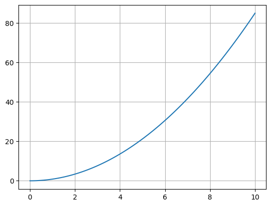
6、弹簧系统每隔1ms周期的系统状态
$$Mx+bx+kx=F$$,试用odeint()对该系统进行求解并作图，其中参数M, k, b, F = 1.0, 0.5, 0.2, 1.0；初值init_status = -1, 0.0；t = np.arange(0, 50, 0.02)。

import numpy as np
import matplotlib.pyplot as plt
from scipy.integrate import odeint

def diff(y, x):
    return np.array(1.7 * x)
# 上面定义的函数在odeint里面体现的就是dy/dx = x
x = np.linspace(0, 10, 100)  # 给出x范围
y = odeint(diff, 0, x)  # 设初值为0 此时y为一个数组，元素为不同x对应的y值
# 也可以直接y = odeint(lambda y, x: x, 0, x)
plt.plot(x, y[:, 0])  # y数组（矩阵）的第一列，（因为维度相同，plt.plot(x, y)效果相同）
plt.grid()
plt.show()  

​

​

7、从参数为1的伽马分布生成1000个随机数,然后绘制这些样点的直方图。你能够在其上绘制此伽马分布的pdf吗(应该匹配)？(参见课件)

shape, scale = 2., 2.  # mean=4, std=2*sqrt(2)
s = np.random.default_rng().gamma(shape, scale, 1000)
import matplotlib.pyplot as plt
import scipy.special as sps  
count, bins, ignored = plt.hist(s, 50, density=True)
y = bins**(shape-1)*(np.exp(-bins/scale) /  
                     (sps.gamma(shape)*scale**shape))
plt.plot(bins, y, linewidth=2, color='r')  
plt.show()

​

​

8、scipy.sparse中提供了多种表示稀疏矩阵的格式，试用dok_martix，lil_matrix表示表示的矩阵[[3 0 8 0] [0 2 0 0] [0 0 0 0] [0 0 0 1]]，并与sparse.coo_matrix表示法进行比较。

import numpy as np
from scipy.sparse import dok_matrix
a = np.matrix([[3,0,8,0],[0,2,0,0],[0,0,0,0],[0,0,0,1]])
S = dok_matrix(a, dtype=np.float32)
for i in range(4):
    for j in range(4):
        S[i, j] = i + j
print(S.toarray())

[[0. 1. 2. 3.]
 [1. 2. 3. 4.]
 [2. 3. 4. 5.]
 [3. 4. 5. 6.]]