CytoTRACE2可视化进阶(修改坐标维持umap图前后一致)

上一期推文已经简单说明了CytoTRACE2的分析流程、注意事项和可视化。

CytoTRACE2单细胞分化潜力预测工具学习：https://mp.weixin.qq.com/s/inF9iGy2X9D2CZLzQBtRdw

有小伙伴观察到使用CytoTRACE2之后的图形会与原始的umap图有些许的不同，虽然在实际应用的时候这种情况是无伤大雅的。

但既然提出了问题，笔者就尝试着去解决一下~

步骤流程

1、导入

rm(list=ls())
library(tidyverse)
library(CytoTRACE2) 
library(Seurat)
library(paletteer)
library(BiocParallel)
register(MulticoreParam(workers = 4, progressbar = TRUE))

load("scRNA.Rdata")
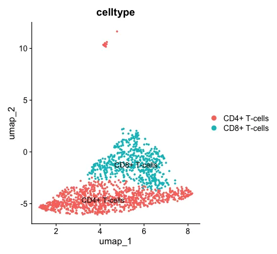
sub_dat <- subset(scRNA, subset = celltype %in% c("CD8+ T-cells", "CD4+ T-cells"))
DimPlot(sub_dat,label = T)

2、提取数据/运行CytoTRACE2

# 提取表达矩阵信息
expression_data <- GetAssayData(sub_dat,layer = "counts")

# 运行CytoTRACE2
cytotrace2_result <- cytotrace2(expression_data,species = 'human')

# 提取注释信息
annotation <- data.frame(phenotype = sub_dat@meta.data$celltype) %>% 
  set_rownames(., colnames(sub_dat))

# 使用plotData函数生成预测和表型关联图
plots <- plotData(cytotrace2_result = cytotrace2_result, 
                  annotation = annotation,
                  expression_data = expression_data
)

3、坐标修改

umap_raw <- as.data.frame(sub_dat@reductions$umap@cell.embeddings) # 为后面修改坐标有用
# 创建一个包含所有需要更新的 plot 名称的向量
plot_names <- c("CytoTRACE2_UMAP", "CytoTRACE2_Potency_UMAP", 
                "CytoTRACE2_Relative_UMAP", "Phenotype_UMAP" 
)
# 循环遍历每个plot并更新坐标
for (plot_name in plot_names) {
  if (!is.null(plots[[plot_name]][[1]]$data)) {
    plots[[plot_name]][[1]]$data$umap_1 <- umap_raw$umap_1
    plots[[plot_name]][[1]]$data$umap_2 <- umap_raw$umap_2
  }
}

# 了解数据类型
class(plots$CytoTRACE2_UMAP[[1]]) 
# [1] "gg"     "ggplot"
class(plots$CytoTRACE2_Potency_UMAP[[1]]) 
# [1] "gg"     "ggplot"
class(plots$CytoTRACE2_Relative_UMAP[[1]]) 
# [1] "gg"     "ggplot"
class(plots$Phenotype_UMAP[[1]])
# [1] "gg"     "ggplot"

# 确认umap的数据范围
x_limits <- range(umap_raw$umap_1, na.rm = TRUE)
y_limits <- range(umap_raw$umap_2, na.rm = TRUE)

# 导出图片
plots$CytoTRACE2_UMAP[[1]] <- plots$CytoTRACE2_UMAP[[1]] + 
  scale_x_continuous(limits = x_limits) + 
  scale_y_continuous(limits = y_limits)
plots$CytoTRACE2_UMAP

plots$CytoTRACE2_Potency_UMAP[[1]] <- plots$CytoTRACE2_Potency_UMAP[[1]] + 
  coord_cartesian(xlim = x_limits, ylim = y_limits)
plots$CytoTRACE2_Potency_UMAP

plots$CytoTRACE2_Relative_UMAP[[1]] <- plots$CytoTRACE2_Relative_UMAP[[1]] + 
  coord_cartesian(xlim = x_limits, ylim = y_limits)
plots$CytoTRACE2_Relative_UMAP

plots$Phenotype_UMAP[[1]] <- plots$Phenotype_UMAP[[1]] + 
  coord_cartesian(xlim = x_limits, ylim = y_limits)
plots$Phenotype_UMAP

library(patchwork)
# 拼接为2x2布局
combined_plot <- (p1[[1]] | p2[[1]]) / (p3[[1]] | p4[[1]])
# 显示拼接后的图形
combined_plot
ggsave("combined_plot.png", plot = combined_plot, width = 10, height = 10)

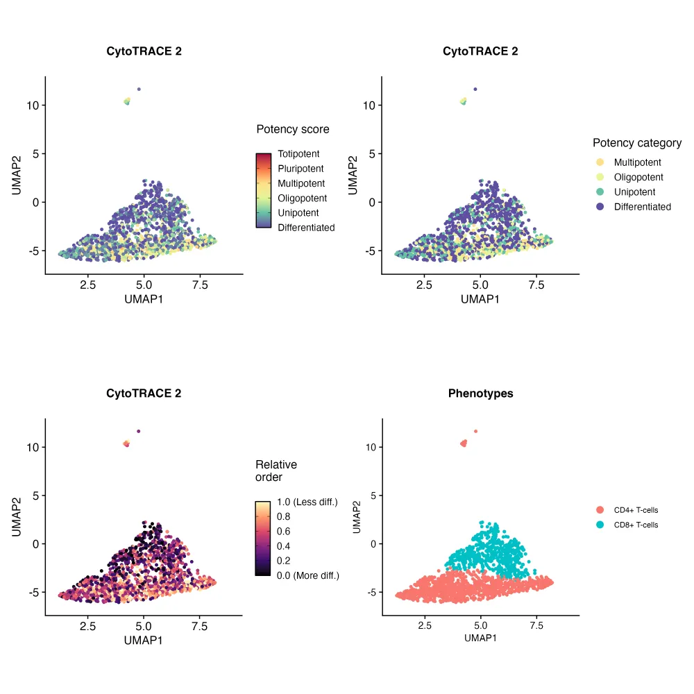
对比之前的结果，是不是新的很棒~

但是笔者不明白的是每次图片导出的时候需要调试下面的两种缩放坐标轴的代码，如果自行使用的时候遇到图片显示不全的情况，就用另一种试一试。

第一种：

coord_cartesian(xlim = x_limits, ylim = y_limits)

第二种：

scale_x_continuous(limits = x_limits) + scale_y_continuous(limits = y_limits)

注：若对内容有疑惑或者有发现明确错误的朋友，请联系后台(欢迎交流)。更多内容可关注公众号：生信方舟

- END -