CMap数据库学习及结果可视化

最新推荐文章于 2024-10-22 23:12:06 发布

凑齐六个字吧

最新推荐文章于 2024-10-22 23:12:06 发布

阅读量3k

点赞数 30

分类专栏：分析工具文章标签：数据库数据分析

本文链接：https://blog.csdn.net/zfyyzhys/article/details/141673403

版权

分析工具专栏收录该内容

43 篇文章

订阅专栏

CMap（Connectivity Map，连接图谱）

CMap是一个生物信息学数据库和工具，旨在通过比较基因表达谱来揭示药物、基因和疾病之间的潜在关联。CMap数据库主要用于寻找药物、化合物和生物过程之间的关系，并用于药物重定位（drug repurposing）和疾病机制研究。

数据来源：不同细胞系；

数据结果：采用的蛋白质层面的数据和小分子药物之间的扰动关系；

数据含量：包含超过150万(这里应该是指不同刺激/条件下的信息数量？)条基因表达谱的库，这些表达谱来自约5000种小分子化合物和约3000种基因试剂，并在多种细胞类型中进行了测试。

这是分析平台的网址：https://clue.io/about

主要功能和用途：

1. 药物重定位（Drug Repurposing）:

CMap 可以帮助研究人员发现已有药物的新的治疗用途。通过将已知药物的基因表达特征与疾病的基因表达特征进行比较，可以识别出可能对该疾病有效的现有药物。

2. 理解药物机制（Mechanism of Action, MoA）:

CMap 允许研究人员通过分析药物处理后的基因表达变化，探索药物的作用机制。通过与已知的作用机制进行比较，可以预测未知化合物的作用方式。

3. 揭示基因功能和病理学机制:

通过将特定基因的基因敲除或过表达实验的基因表达谱与 CMap 数据库中的药物处理基因表达谱进行比较，研究人员可以推断出该基因在特定生物过程中或疾病中的作用。

4. 疾病关联研究:

CMap 可以用于研究不同疾病的分子机制。通过比较不同疾病的基因表达特征，可以识别出与特定疾病相关的分子标志物或潜在的治疗靶点。

5. 化合物筛选:

研究人员可以利用 CMap 数据库进行化合物筛选，找到能够逆转某些疾病相关基因表达模式的候选化合物，从而为新药开发提供线索。

工作原理：

CMap 数据库的核心是大量的基因表达谱，这些表达谱是通过微阵列或 RNA-seq 技术获得的，记录了细胞在不同化合物、基因干扰或基因过表达处理后的基因表达变化。研究人员可以输入一个基因表达谱（如某种疾病的差异基因谱），然后网站会根据表达谱信息富集得到相关性分数(-100 ~ 100)进而识别潜在的敏感性药物。同时该相关性分数越小则差异药物的敏感性可能越强(可以规定小于-95为潜在治疗性药物) 。

网页及代码分析流程

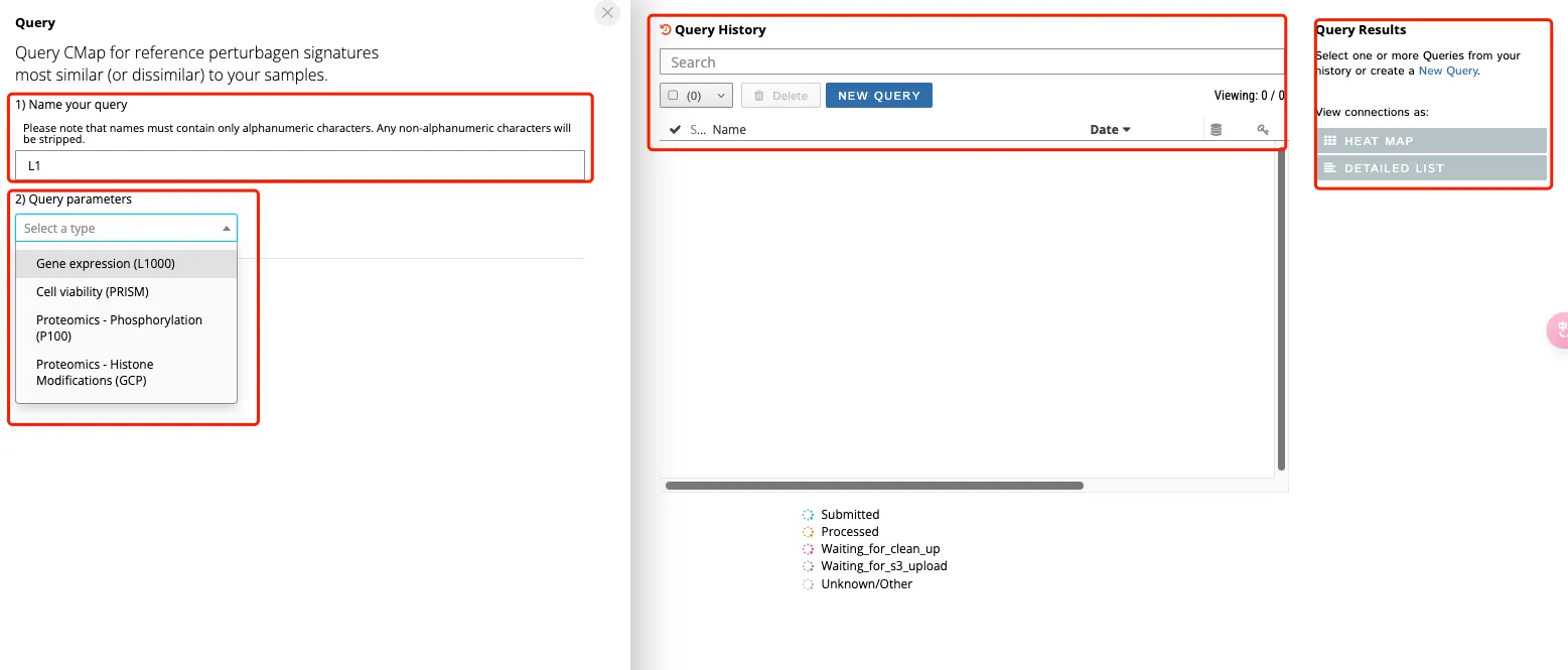
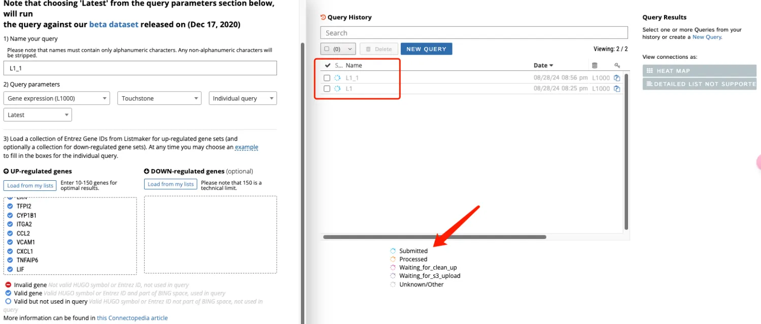
1、进入官网(https://clue.io/)，注册登录后点击tools中的Query(主要用这个，其他的可自行探索)

2、查看工作界面

左侧(1)红框代表设置的项目名称；(2)红框代表选择上传数据的情况，一般来说都是gene expression。如果输入的事蛋白组的数据，就可以选择Proteomics的选项，总之要根据自己的数据类型而决定。

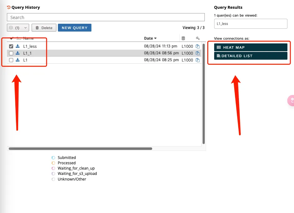
右侧第一个框可以搜索既往分析的结果，第二个的选项可以进行数据展示。

3、选择了gene expression之后还需要进行参数设置和上传上下调差异基因。参数设置一般默认即可，其中Latest中还有1.0的老版本，建议选择1.0的老版本！如果选择1.0的版本可以在网页上生成热图和数据的detail list。

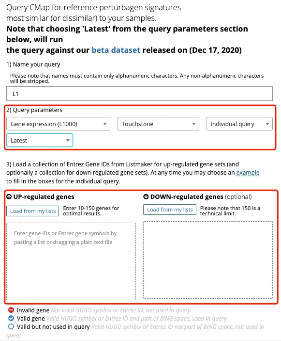
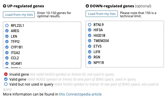
4、输入基因之后还可以根据圆圈的颜色样式告诉使用者该基因是否可以被查询。在这里的上下调栏中各有一个基因是正确的但是在这个数据库中没有信息。此外，输入基因的数量最少是10个，最多不能超过150个，下调基因可以不输入。

5、支持多任务同时上传并分析

6、如果显示Detailed list not supported，那就直接下载全部的数据。如果Detailed list可以点击就进入页面导出所需要的数据即可。

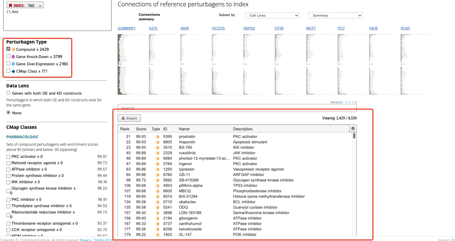
7、点击Compound选项，然后导出信息。

8、代码环节

加载数据，提取上下调各排名前150的差异基因。

rm(list = ls())
degs <- read.csv("degs.csv",row.names = 1,header = T)
head(degs)[1:4,1:4]
#           logFC   AveExpr        t      P.Value
# CTSL   1.328398 10.114151 14.95486 1.120455e-25
# ARNTL2 1.126544  6.885511 12.53450 3.969902e-21
# NOP16  1.199536  7.485119 12.29963 1.137443e-20
# SRXN1  1.074733  8.582499 12.24155 1.476961e-20
 
up_150 <- rownames(tail(degs[order(degs$logFC),],150))
down_150 <- rownames(head(degs[order(degs$logFC),],150))
write.table(up_150,file = "up_150.txt",append = F,quote = T,sep = "",row.names = T,col.names = T)
write.table(down_150,file = "up_150.txt",append = F,quote = T,sep = "",row.names = T,col.names = T)

读取export数据

# 记住 要选择负值！！负值！！
library(data.table)
res <- fread("export.txt",,data.table = F)
head(res)
#   Rank Score Type            ID                            Name         Description
# 1   21 99.93   cp BRD-K91145395                      prostratin       PKC activator
# 2   22 99.93   cp BRD-K10098805                       rhapontin Apoptosis stimulant
# 3   23 99.93   cp BRD-K47983010                          BX-795       IKK inhibitor
# 4   45 99.89   cp BRD-K53972329                     ruxolitinib       JAK inhibitor
# 5   46 99.89   cp BRD-A15079084 phorbol-12-myristate-13-acetate       PKC activator
# 6   47 99.89   cp BRD-A52650764                         ingenol       PKC activator

# 首先对 res 按照 Score 列进行排序
res_sorted <- res[order(res$Score, decreasing = TRUE), ]
# 然后选择第2列、第5列和第6列，并取前50行
res_tail50 <- tail(res_sorted[, c(2, 5, 6)], 50)
write.csv(res_tail50,"res_tail50.scv")

# 也可以按照药物名称
matches <- grep("Endothelin|Phosphodiesterase|Prostacyclin|guanosine|calcium", res$Description)
M <- res[matches,]
write.csv(M,"matches.scv")

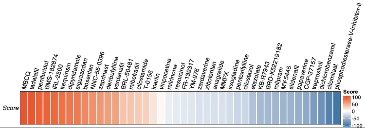
热图

M <- M[,c("Name","Score","Description")]
# 移除现有的行名（如果有）
rownames(M) <- NULL
mydata <- M[,-3]%>%
  column_to_rownames('Name')

library(circlize)
library(ComplexHeatmap)
library(pheatmap)
col_fun = colorRamp2(c(-100, 0, 100), c("#2978AB", "white", "#FF410DCC"))

Heatmap(as.matrix(t(mydata)), 
        col = col_fun, 
        rect_gp = gpar(col = "white", lwd = 2),
        name = "Score",
        show_row_dend = FALSE, 
        show_column_dend = FALSE,
        show_column_names = TRUE, 
        column_names_side  = 'top',
        column_names_rot= 75,
        row_names_gp = gpar(fontsize = 12, fontface="italic"),
        show_row_names = TRUE,
        row_names_side = 'left',
        na_col = "white", 
        cluster_rows =  F, 
        cluster_columns = T,border = 'black',
        heatmap_legend_param = list(grid_width = unit(0.5, "cm"),
                                    grid_height = unit(1.5, "cm")))
library(export)
graph2pdf(file=paste0('heatmap.pdf'),width = 10,height = 3.5)
dev.off()

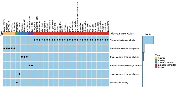
潜在治疗性药物的作用模式图(OncoPrint函数)

input_raw <- res[res$Name%in%rownames(mydata),c(6,5)]  
input <- reshape2::dcast(input_raw, Description ~ Name)
# Description ~ Name：
# 这是一个公式，用于指定“宽格式”中的行和列：
# Description：指定将作为“宽格式”数据的行标识符的变量。
# Name：指定将作为“宽格式”数据的列名的变量。
# 这意味着dcast会将input数据框中具有相同Description的行聚合在一起，并为每个Name创建单独的列。
rownames(input) <- input$Description 
input <- input[, -1] 
input <- as.matrix(input)

input[!is.na(input)] <- "inhibitor"
input[is.na(input)] <- ""
input <- input[, order(colnames(input))]

pp <- as.data.frame(input)
pp <- data.frame(Name=colnames(pp),Type=1:42) #这里的Type数量要跟着colnames数量走
dd <- merge(input_raw,pp,by.x = 2,by.y=1)
# 这些参数指定了用于合并的键列。
# by.x = 2：表示使用 input 数据框的第2列作为合并的键。
# by.y = 1：表示使用 pp 数据框的第1列作为合并的键。
dd$Type[dd$Description%like%'inhibitor'] <- "Inhibitor"
dd$Type[dd$Description%like%'agonist'] <- "Agonist"
dd$Type[dd$Description%like%'channel blocker'] <- "Channel blocker"
dd$Type[dd$Description%like%'exchange inhibitor'] <- "Exchange inhibitor"
dd$Type[dd$Description%like%'analog'] <- "Analog"
dd<- dd[order(dd$Type,decreasing = F),]
alter_fun = list(
  background = function(x, y, w, h) 
    grid.rect(x, y, w*0.9, h*0.9, gp = gpar(fill = "skyblue", col = "grey")),
  # dots
  inhibitor = function(x, y, w, h) 
    grid.points(x, y, pch = 16, size = unit(0.8, "char"))
  
)
#ha_coldata <- colSums(apply(oncoprintinput, 2, function(x) x=="inhibitor") + 0) %>% as.numeric()
# 这里输入的事input，input中文字信息都改成了inhibitor，因此可以做计算
ha_rowdata <- rowSums(apply(input, 2, function(x) x=="inhibitor") + 0) %>% as.numeric() 
table(dd$Type)
# dd$Type <- factor(dd$Type,levels = c("Agonist","Analog","Channel blocker",
#                                 "Exchange inhibitor","Inhibitor"))
top_ha <- HeatmapAnnotation(Type = dd[,3], 
                            col = list(Type = c("Agonist" = "#FDBF6F",#1666A5
                                                "Analog" = "#33A02C",
                                                "Channel blocker" = "#1F78B4",#B5CEE0
                                                "Exchange inhibitor" = "#6A3D9A",
                                                'Inhibitor'='#E31A1C')),#F7E897FF
                            show_legend = T,#是否要显示annotation legend
                            annotation_height = unit(30, "mm"),#临床annotation的高度
                            #annotation_legend_param = list(Type = list(title = "Type")),
                            annotation_name_side = "left",
                            annotation_name_rot = 90)
right_ha <- rowAnnotation(count = anno_barplot(ha_rowdata, axis = F, border = F, 
                                               gp = gpar(fill = "skyblue"),
                                               bar_width = 1, width = unit(2, "cm")),
                          annotation_name_side = "top",
                          annotation_name_rot = 0)

# 调整 input 中的列顺序与 dd 中的顺序一致
column_order <- intersect(dd$Name,colnames(input))
input <- input[,column_order]
#oncoprint 是一种通过热图的方式来可视化多个基因组变异事件。ComplexHeatmap 包提供了 oncoPrint() 函数来绘制这种类型的图。
oncoPrint(input, alter_fun = alter_fun, 
          show_column_names = TRUE, 
          column_names_side = "top",
          column_order = column_order, 
          top_annotation = top_ha,
          right_annotation = right_ha,
          show_pct = F, 
          show_heatmap_legend = F)
decorate_annotation("Type", {
  grid.text("Mechanism of Action", unit(1, "npc") + unit(3, "mm"), just = "left")})

graph2pdf(file=paste0('oncoPrint.pdf'),width = 12,height = 6)
dev.off()