


在市场调研的广阔天地中,“正大杯”全国大学生市场调查与分析大赛一直是创新与实践的沃土。众多参赛作品中,聚类分析作为一种重要的统计工具,被广泛应用于揭示客户群体的内在结构和行为模式。这种方法不仅帮助参赛者深入理解数据,更在多个获奖作品中发挥了关键作用。例如
国家一等奖作品:《“药香浮古韵,新茶溢清芬”——上海市年轻居民对新中式养生饮品消费的市场现状以及偏好调查》
作品简介:作品通过网络评论分析和问卷调查,探索消费者对新中式养生饮品的关注、并通过人群聚类和结构方程模型探明购买动机。提出针对不同消费者群体的营销建议,助力企业在竞争中脱颖而出。
国家一等奖作品:《川渝茶缘浓,巴适学子心——当代大学生对于现制茶饮消费需求调研及新店开业推广方案》
作品简介:作品利用SWOT分析明确川渝地区大学生为调研目标群体;借助调查问卷、Logistic回归分析、K-means聚类分析与SICAS模型将目标群体进行类别划分并针对性研究其消费习惯和对茶饮产品的核心需求;4P营销策略针对消费者不同方面的需求提供了可行性建议;解决开店时“卖给谁、卖什么、怎么卖”的问题。
客户群体聚类分析案项目实战

在这个项目中,我们将对杂货公司数据库中的客户记录进行无监督的数据聚类。客户细分是将客户分为反映每个集群中客户之间相似性的组的做法。我们会将客户进行细分,以优化每个客户对业务的重要性。根据客户的不同需求和行为修改产品。它还有助于企业满足不同类型客户的担忧。
导入库
#Importing the Libraries
import numpy as np
import pandas as pd
import datetime
import matplotlib
import matplotlib.pyplot as plt
from matplotlib import colors
import seaborn as sns
from sklearn.preprocessing import LabelEncoder
from sklearn.preprocessing import StandardScaler
from sklearn.decomposition import PCA
from yellowbrick.cluster import KElbowVisualizer
from sklearn.cluster import KMeans
import matplotlib.pyplot as plt, numpy as np
from mpl_toolkits.mplot3d import Axes3D
from sklearn.cluster import AgglomerativeClustering
from matplotlib.colors import ListedColormap
from sklearn import metrics
import warnings
import sys
if not sys.warnoptions:
    warnings.simplefilter("ignore")
np.random.seed(42)
加载数据
#Loading the dataset
data = pd.read_csv("../input/customer-personality-analysis/marketing_campaign.csv", sep="\t")
print("Number of datapoints:", len(data))
data.head()

数据清洗
#Information on features
data.info()
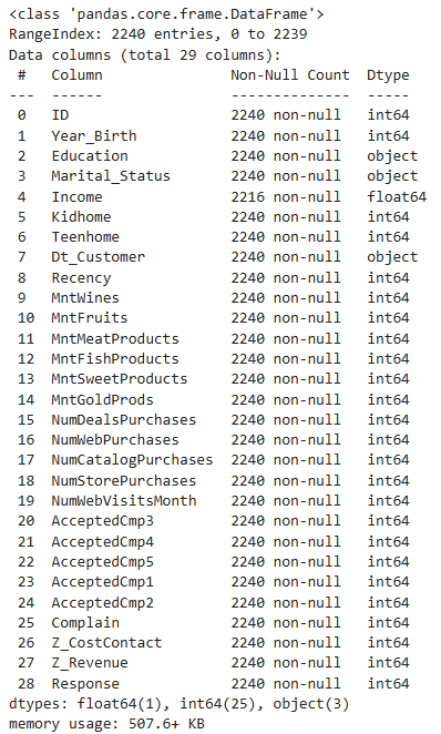
从上面的输出中,我们可以得出结论并注意到:
- 收入中存在缺失值
- 指示客户加入数据库的日期的 Dt_Customer 不会被解析为 DateTime
- 我们的数据框中有一些分类特征;因为 dtype: object 中有一些功能)。所以我们稍后需要将它们编码为数字形式。
首先,对于缺失值,我只需删除具有缺失收入值的行。
#To remove the NA values
data = data.dropna()
print("The total number of data-points after removing the rows with missing values are:", len(data))
在下一步中,我将根据“Dt_Customer”创建一个功能,指示客户在公司数据库中注册的天数。然而,为了简单起见,我将这个值相对于记录中的最新客户。
因此,为了获取值,我必须检查最新和最旧的记录日期。
data["Dt_Customer"] = pd.to_datetime(data["Dt_Customer"])
dates = []
for i in data["Dt_Customer"]:
    i = i.date()
    dates.append(i)
#Dates of the newest and oldest recorded customer
print("The newest customer's enrolment date in therecords:",max(dates))
print("The oldest customer's enrolment date in the records:",min(dates))
创建相对于上次记录日期顾客开始在商店购物的天数的特征(“Customer_For”)
#Created a feature "Customer_For"
days = []
d1 = max(dates) #taking it to be the newest customer
for i in dates:
    delta = d1 - i
    days.append(delta)
data["Customer_For"] = days
data["Customer_For"] = pd.to_numeric(data["Customer_For"], errors="coerce")
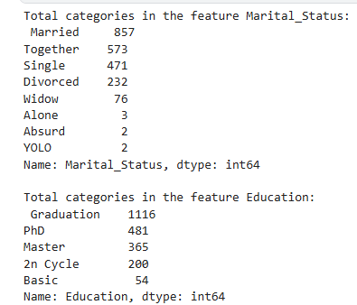
现在我们将探索分类特征中的唯一值,以清楚地了解数据。
print("Total categories in the feature Marital_Status:\n", data["Marital_Status"].value_counts(), "\n")
print("Total categories in the feature Education:\n", data["Education"].value_counts())
接下来,我将执行以下步骤来设计一些新功能:
- 通过指示相应人的出生年份的“Year_Birth”提取客户的“Age”。
- 创建另一个特征“Spent”,指示客户在两年内在各个类别中花费的总金额。
- 在“Marital_Status”的基础上创建另一个特征“Living_With”来提取夫妻的生活状况。
- 创建“Children”特征来指示家庭中的儿童总数,即儿童和青少年。
- 为了进一步明确家庭情况,创建指示“Family_Size”的特征
- 创建一个特征“Is_Parent”来指示父母身份
- 最后,我将通过简化其值计数在“Education”中创建三个类别。
- 删除一些多余的功能
#Feature Engineering
#Age of customer today
data["Age"] = 2021-data["Year_Birth"]

#Total spendings on various items
data["Spent"] = data["MntWines"]+ data["MntFruits"]+ data["MntMeatProducts"]+ data["MntFishProducts"]+ data["MntSweetProducts"]+ data["MntGoldProds"]

#Deriving living situation by marital status"Alone"
data["Living_With"]=data["Marital_Status"].replace({"Married":"Partner", "Together":"Partner", "Absurd":"Alone", "Widow":"Alone", "YOLO":"Alone", "Divorced":"Alone", "Single":"Alone",})
#Feature indicating total children living in the household
data["Children"]=data["Kidhome"]+data["Teenhome"]
#Feature for total members in the householde
data["Family_Size"] = data["Living_With"].replace({"Alone": 1, "Partner":2})+ data["Children"]
#Feature pertaining parenthood
data["Is_Parent"] = np.where(data.Children> 0, 1, 0)
#Segmenting education levels in three groups
data["Education"]=data["Education"].replace({"Basic":"Undergraduate","2n Cycle":"Undergraduate", "Graduation":"Graduate", "Master":"Postgraduate", "PhD":"Postgraduate"})
#For clarity
data=data.rename(columns={"MntWines": "Wines","MntFruits":"Fruits","MntMeatProducts":"Meat","MntFishProducts":"Fish","MntSweetProducts":"Sweets","MntGoldProds":"Gold"})
#Dropping some of the redundant features
to_drop = ["Marital_Status", "Dt_Customer", "Z_CostContact", "Z_Revenue", "Year_Birth", "ID"]
data = data.drop(to_drop, axis=1)
可视化数据
#To plot some selected features
#Setting up colors prefrences
sns.set(rc={"axes.facecolor":"#FFF9ED","figure.facecolor":"#FFF9ED"})
pallet = ["#682F2F", "#9E726F", "#D6B2B1", "#B9C0C9", "#9F8A78", "#F3AB60"]
cmap = colors.ListedColormap(["#682F2F", "#9E726F", "#D6B2B1", "#B9C0C9", "#9F8A78", "#F3AB60"])
#Plotting following features
To_Plot = [ "Income", "Recency", "Customer_For", "Age", "Spent", "Is_Parent"]
print("Reletive Plot Of Some Selected Features: A Data Subset")
plt.figure()
sns.pairplot(data[To_Plot], hue= "Is_Parent",palette= (["#682F2F","#F3AB60"]))
#Taking hue
plt.show()
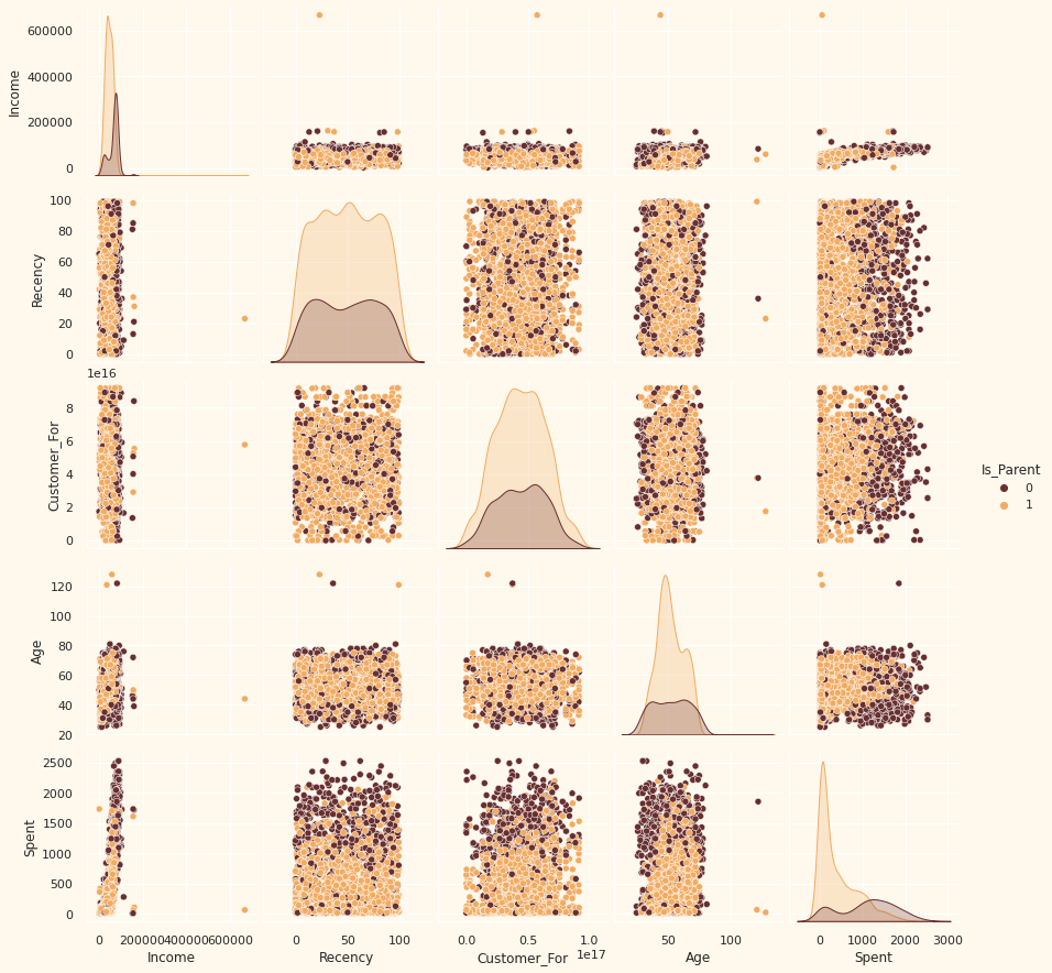
图解:显然,收入和年龄特征存在一些异常值。我们将删除数据中的异常值。
#Dropping the outliers by setting a cap on Age and income.
data = data[(data["Age"]<90)]
data = data[(data["Income"]<600000)]
print("The total number of data-points after removing the outliers are:", len(data))
接下来,让我们看看特征之间的相关性。 (此时不包括分类属性)
#correlation matrix
corrmat= data.corr()
plt.figure(figsize=(20,20))
sns.heatmap(corrmat,annot=True, cmap=cmap, center=0)
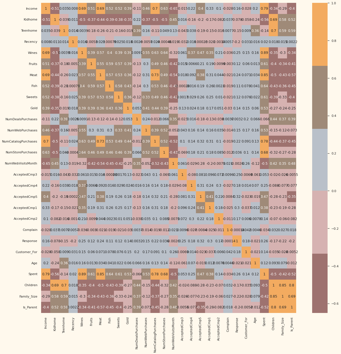
图解:数据相当干净,并且包含了新功能。我们将继续下一步。也就是对数据进行预处理。
数据预处理
在本节中,我们将预处理数据以执行聚类操作。应用以下步骤对数据进行预处理:
- 对分类特征进行标签编码
- 使用标准缩放器缩放功能
- 创建子集数据框以进行降维
#Get list of categorical variables
s = (data.dtypes == 'object')
object_cols = list(s[s].index)

print("Categorical variables in the dataset:", object_cols)
Categorical variables in the dataset: ['Education', 'Living_With']
#Label Encoding the object dtypes.
LE=LabelEncoder()
for i in object_cols:
    data[i]=data[[i]].apply(LE.fit_transform)

print("All features are now numerical")
All features are now numerical
#Creating a copy of data
ds = data.copy()
# creating a subset of dataframe by dropping the features on deals accepted and promotions
cols_del = ['AcceptedCmp3', 'AcceptedCmp4', 'AcceptedCmp5', 'AcceptedCmp1','AcceptedCmp2', 'Complain', 'Response']
ds = ds.drop(cols_del, axis=1)
#Scaling
scaler = StandardScaler()
scaler.fit(ds)
scaled_ds = pd.DataFrame(scaler.transform(ds),columns= ds.columns )
print("All features are now scaled")
All features are now scaled
#Scaled data to be used for reducing the dimensionality
print("Dataframe to be used for further modelling:")
scaled_ds.head()
数据降维
在这个问题中,最终分类的依据有很多因素。这些因素基本上是属性或特征。特征数量越多,使用起来就越困难。其中许多特征是相关的,因此是多余的。这就是为什么我们将在将所选特征放入分类器之前对它们进行降维。降维是通过获得一组主变量来减少所考虑的随机变量数量的过程。
主成分分析 (PCA) 是一种降低此类数据集维度、提高可解释性但同时最大限度减少信息丢失的技术。
本节中的步骤:
- 使用 PCA 降维
- 绘制简化后的数据框
- 使用 PCA 降维
- 对于这个项目,我们将把尺寸减少到 3。
#Initiating PCA to reduce dimentions aka features to 3
pca = PCA(n_components=3)
pca.fit(scaled_ds)
PCA_ds = pd.DataFrame(pca.transform(scaled_ds), columns=(["col1","col2", "col3"]))
PCA_ds.describe().T
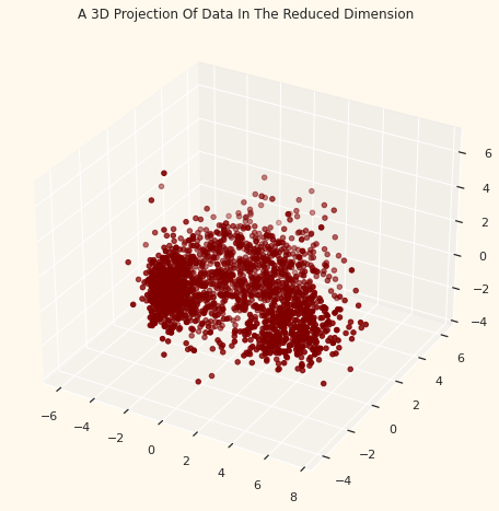
#A 3D Projection Of Data In The Reduced Dimension
x =PCA_ds["col1"]
y =PCA_ds["col2"]
z =PCA_ds["col3"]
#To plot
fig = plt.figure(figsize=(10,8))
ax = fig.add_subplot(111, projection="3d")
ax.scatter(x,y,z, c="maroon", marker="o" )
ax.set_title("A 3D Projection Of Data In The Reduced Dimension")
plt.show()
聚类分析
现在我们已将属性减少到三个维度,我将通过聚合聚类(Agglomerative clustering)来执行聚类。Agglomerative clustering是一种层次聚类方法。它涉及合并示例,直到达到所需的集群数量。
聚类涉及的步骤:
- 肘部法(Elbow)确定要形成的簇的数量
- 通过聚合聚类进行聚类
- 检查通过散点图形成的簇
# Quick examination of elbow method to find numbers of clusters to make.
print('Elbow Method to determine the number of clusters to be formed:')
Elbow_M = KElbowVisualizer(KMeans(), k=10)
Elbow_M.fit(PCA_ds)
Elbow_M.show()
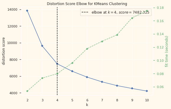
图解:上面的单元格表明四个将是该数据的最佳簇数。接下来,我们将拟合聚合聚类模型以获得最终的聚类。
#Initiating the Agglomerative Clustering model
AC = AgglomerativeClustering(n_clusters=4)
# fit model and predict clusters
yhat_AC = AC.fit_predict(PCA_ds)
PCA_ds["Clusters"] = yhat_AC
#Adding the Clusters feature to the orignal dataframe.
data["Clusters"]= yhat_AC
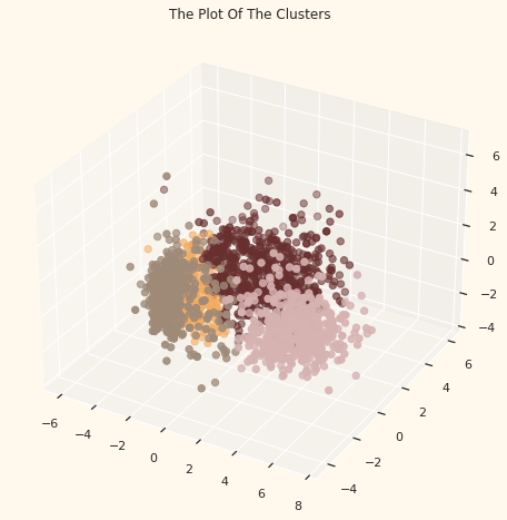
为了检查形成的簇,让我们看一下簇的 3-D 分布。
#Plotting the clusters
fig = plt.figure(figsize=(10,8))
ax = plt.subplot(111, projection='3d', label="bla")
ax.scatter(x, y, z, s=40, c=PCA_ds["Clusters"], marker='o', cmap = cmap )
ax.set_title("The Plot Of The Clusters")
plt.show()
评估模型
因为这是一个无监督的聚类。我们没有标记功能来评估或评分我们的模型。本节的目的是研究形成的簇中的模式并确定簇模式的性质。
为此,我们将通过探索性数据分析并得出结论,根据集群来查看数据。首先我们看一下cluster的分组分布
#Plotting countplot of clusters
pal = ["#682F2F","#B9C0C9", "#9F8A78","#F3AB60"]
pl = sns.countplot(x=data["Clusters"], palette= pal)
pl.set_title("Distribution Of The Clusters")
plt.show()
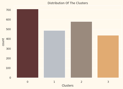
图解:这些簇似乎分布相当均匀。
pl = sns.scatterplot(data = data,x=data["Spent"], y=data["Income"],hue=data["Clusters"], palette= pal)
pl.set_title("Cluster's Profile Based On Income And Spending")
plt.legend()
plt.show()
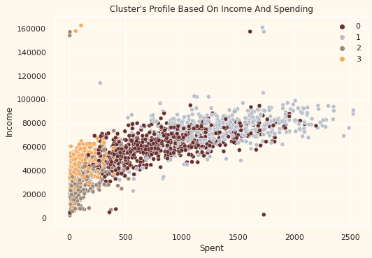
图解:收入与支出图显示集群模式
- 第 0 组:高支出和平均收入
- 第一组:高支出和高收入
- 第二组:低支出和低收入
- 第三组:高支出和低收入
接下来,我将根据数据中的各种产品查看集群的详细分布。即:酒、水果、肉、鱼、糖果和黄金
plt.figure()
pl=sns.swarmplot(x=data["Clusters"], y=data["Spent"], color= "#CBEDDD", alpha=0.5 )
pl=sns.boxenplot(x=data["Clusters"], y=data["Spent"], palette=pal)
plt.show()
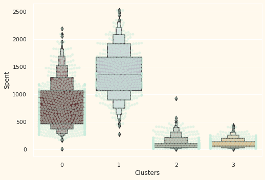
图解:从上图可以清楚地看出,集群1 是我们最大的客户群,紧随其后的是集群 0。我们可以探索每个集群在有针对性的营销策略方面的支出。
接下来让我们探讨一下我们的活动过去的表现如何。
#Creating a feature to get a sum of accepted promotions
data["Total_Promos"] = data["AcceptedCmp1"]+ data["AcceptedCmp2"]+ data["AcceptedCmp3"]+ data["AcceptedCmp4"]+ data["AcceptedCmp5"]
#Plotting count of total campaign accepted.
plt.figure()
pl = sns.countplot(x=data["Total_Promos"],hue=data["Clusters"], palette= pal)
pl.set_title("Count Of Promotion Accepted")
pl.set_xlabel("Number Of Total Accepted Promotions")
plt.show()
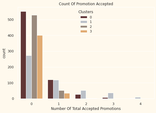
图解:到目前为止,这些活动尚未引起强烈反响。总体参与者很少。而且,没有一个人参与全部5件事。也许需要更有针对性和精心策划的活动来促进销售。
#Plotting the number of deals purchased
plt.figure()
pl=sns.boxenplot(y=data["NumDealsPurchases"],x=data["Clusters"], palette= pal)
pl.set_title("Number of Deals Purchased")
plt.show()
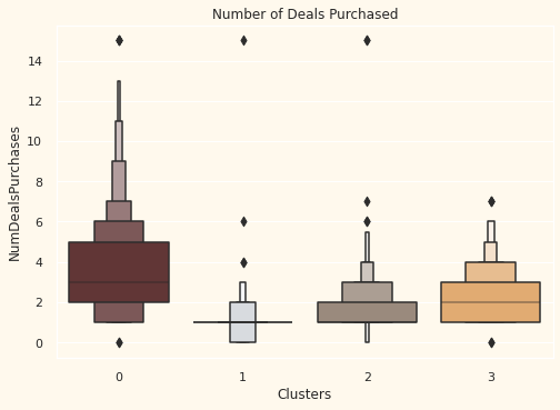
图解:与竞选活动不同的是,所提供的优惠效果很好。集群 0 和集群 3 的结果最好。但是,我们的明星客户集群 1 不太热衷于交易。似乎没有什么能压倒性地吸引集群 2。
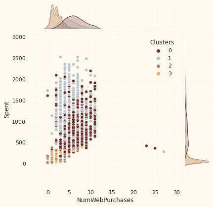
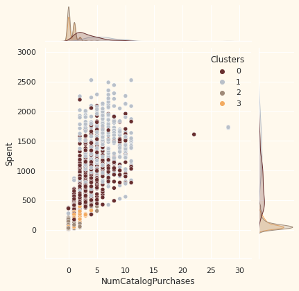
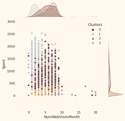
#for more details on the purchasing style
Places =["NumWebPurchases", "NumCatalogPurchases", "NumStorePurchases",  "NumWebVisitsMonth"]

for i in Places:
    plt.figure()
    sns.jointplot(x=data[i],y = data["Spent"],hue=data["Clusters"], palette= pal)
    plt.show()

描述特征
现在我们已经形成了集群并观察了他们的购买习惯。让我们看看这些集群中都有哪些人。为此,我们将对形成的集群进行分析,并得出谁是我们的明星客户以及谁需要零售店营销团队更多关注的结论。
为了决定,我将根据客户所在的集群绘制一些表明客户个人特征的特征。根据结果,我将得出结论。
Personal = [ "Kidhome","Teenhome","Customer_For", "Age", "Children", "Family_Size", "Is_Parent", "Education","Living_With"]

for i in Personal:
    plt.figure()
    sns.jointplot(x=data[i], y=data["Spent"], hue =data["Clusters"], kind="kde", palette=pal)
    plt.show()
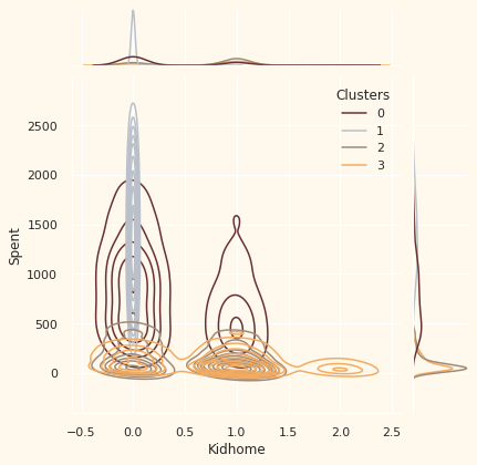
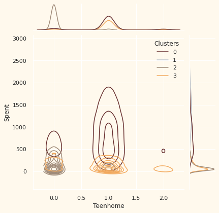
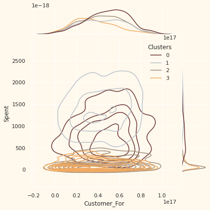
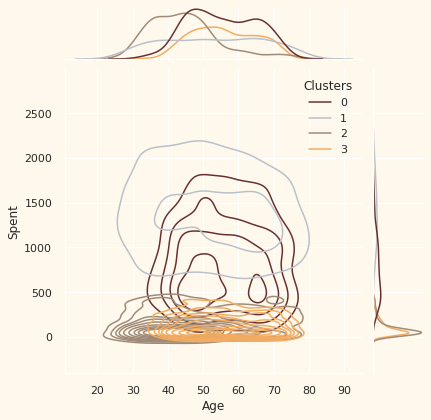
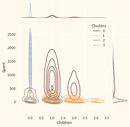
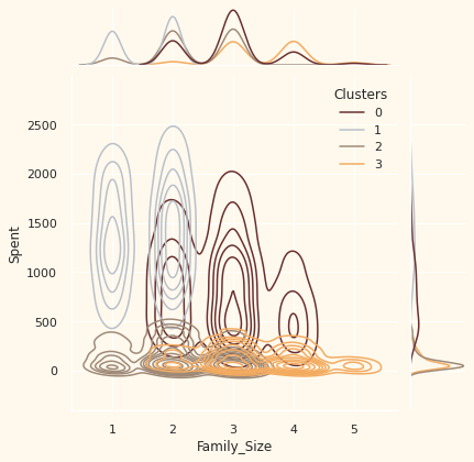
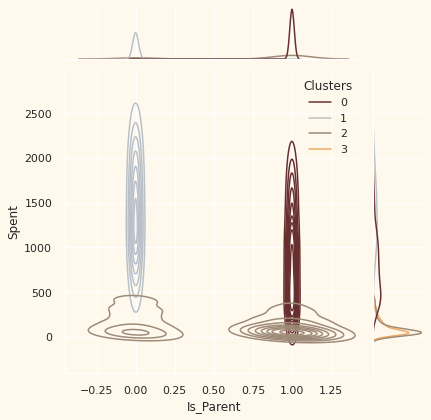
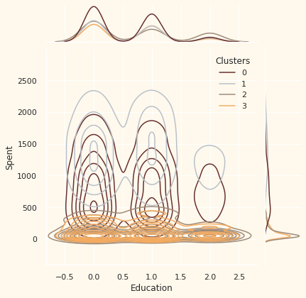
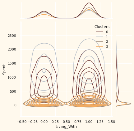
注意事项:
可以推断出以下关于不同集群中的客户的信息。

结论
在这个项目中,我执行了无监督聚类。我确实使用了降维,然后进行了凝聚聚类。我提出了 4 个聚类,并进一步根据家庭结构和收入/支出对聚类中的客户进行分析。这可以用于规划更好的营销策略。


 340
340

 被折叠的 条评论
为什么被折叠?
被折叠的 条评论
为什么被折叠?
 到【灌水乐园】发言


