【pcl入门教程分割系列】之Difference of Normals Based Segmentation

DoN Segmentation

　　之前的博客有过介绍几种地面点云提取or分割的方法，本次博客介绍一下通过差分法线特征(Difference of Normals features, DoN)的方式来进行分割。在pcl源码库中对应的接口函数为pcl::DifferenceOfNormalsEstimation类，该算法对于给定输入点云按照尺度进行分段，来进行查找属于给定比例尺度参数的点集。

DoN理论浅析

　　DoN算法提供一种计算高效、多尺度方式去处理无序的大场景点云数据。算法思想较为简单：对于每一个点$p$在点云数据集$P$中，根于不同的邻域大小来进行计算点$p$的法向量，假设有两个邻域大小(也称作支撑半径)分别为$r_l$与$r_s$，其中$r_l$代表邻域范围较大，$r_s$代表邻域范围较小($r_l>r_s$)；那么点$p$对应的法向量分别为：$\hat{n}(p,r_l)$和$\hat{n}(p,r_s)$。获取不同邻域的法向量之后，对其进行差分运算，即可得到点$p$的差分法向量。公式如下：
$$\Delta \hat{n}(p,r_s,r_l)=\frac{\hat{n}(p,r_s)-\hat{n}(p,r_l)}{2}$$

　　从上述可以看到，$\hat{n}(p,r)$为点$p$的空间法向量估计，在邻域半径为$r$的范围。当然，不同的邻域半径求取的法向量会有比较大的差异，见下图：

　　DoN算法主要是观察在任何给定半径的情况下进行曲面法线估计，反映的是曲面在支撑不同比例半径下的基本几何体。尽管有很多种方法来进行曲面法线的估计，但是法线总是以一个支持半径(或者通过一定数量的邻域点)来进行估计的。这样支持半径就能够确定法线表示在该尺度下的曲面结构。上图在一维情况下简单表述DoN的过程，我们可以看到在小邻域的法线估计$\hat{n}$和切线$T$很容易受到小尺度的表面结构或类似噪声的干扰。另一方面，大邻域的半径估计法线和切线收小尺度结构的干扰较小。

Steps Difference of Normals for Segmentation

1. 对每个点$p$使用比较大的支持半径邻域$r_l$进行法线估计；
2. 对每个点$p$使用比较小的支持半径领域$r_s$进行法线估计；
3. 对每个点按照上述法线差分公式进行计算出每个点的DoN;
4. 按照阈值Threshold过滤生成的向量场以隔离属于所需要感兴趣的尺度/区域。

代码部分

#include <string>
#include <chrono>

#include <pcl/point_types.h>
#include <pcl/io/pcd_io.h>
#include <pcl/search/organized.h>
#include <pcl/search/kdtree.h>
#include <pcl/features/normal_3d_omp.h>
#include <pcl/filters/conditional_removal.h>
// #include <pcl/segmentation/extract_clusters.h>

#include <pcl/features/don.h>

using namespace pcl;

int main (int argc, char *argv[])
{
  ///The smallest scale to use in the DoN filter.
  double scale1;
  ///The largest scale to use in the DoN filter.
  double scale2;
  ///The minimum DoN magnitude to threshold by
  double threshold;

  if (argc < 5)
  {
    std::cerr << "usage: " << argv[0] << " inputfile smallscale largescale threshold segradius" << std::endl;
    exit (EXIT_FAILURE);
  }
  /// the file to read from.
  std::string infile = argv[1];
  /// small scale
  std::istringstream (argv[2]) >> scale1;
  /// large scale
  std::istringstream (argv[3]) >> scale2;
  std::istringstream (argv[4]) >> threshold;   // threshold for DoN magnitude

  // Load cloud in blob format
  pcl::PCLPointCloud2 blob;
  pcl::io::loadPCDFile (infile.c_str (), blob);
  pcl::PointCloud<PointXYZI>::Ptr cloud (new pcl::PointCloud<PointXYZI>);
  pcl::fromPCLPointCloud2 (blob, *cloud);

  auto startTime = std::chrono::steady_clock::now();

  // Create a search tree, use KDTreee for non-organized data.
  pcl::search::Search<PointXYZI>::Ptr tree;
  if (cloud->isOrganized ())
  {
    tree.reset(new pcl::search::OrganizedNeighbor<PointXYZI>());
  }
  else
  {
    tree.reset(new pcl::search::KdTree<PointXYZI>(false));
  }

  // Set the input pointcloud for the search tree
  tree->setInputCloud(cloud);

  if (scale1 >= scale2)
  {
    std::cerr << "Error: Large scale must be > small scale!" << std::endl;
    exit (EXIT_FAILURE);
  }

  // Compute normals using both small and large scales at each point
  pcl::NormalEstimationOMP<PointXYZI, PointNormal> ne;
  ne.setInputCloud(cloud);
  ne.setSearchMethod(tree);

  /**
   * NOTE: setting viewpoint is very important, so that we can ensure
   * normals are all pointed in the same direction!
   */
  ne.setViewPoint(std::numeric_limits<float>::max(), std::numeric_limits<float>::max(), std::numeric_limits<float>::max());

  // calculate normals with the small scale
  std::cout << "Calculating normals for scale..." << scale1 << std::endl;
  pcl::PointCloud<PointNormal>::Ptr normals_small_scale(new pcl::PointCloud<PointNormal>);

  ne.setRadiusSearch(scale1);
  ne.compute(*normals_small_scale);

  // calculate normals with the large scale
  std::cout << "Calculating normals for scale..." << scale2 << std::endl;
  pcl::PointCloud<PointNormal>::Ptr normals_large_scale(new pcl::PointCloud<PointNormal>);

  ne.setRadiusSearch(scale2);
  ne.compute(*normals_large_scale);

  // Create output cloud for DoN results
  PointCloud<PointNormal>::Ptr doncloud(new pcl::PointCloud<PointNormal>);
  copyPointCloud(*cloud, *doncloud);

  std::cout << "Calculating DoN... " << std::endl;
  // Create DoN operator
  pcl::DifferenceOfNormalsEstimation<PointXYZI, PointNormal, PointNormal> don;
  don.setInputCloud(cloud);
  don.setNormalScaleLarge(normals_large_scale);
  don.setNormalScaleSmall(normals_small_scale);

  if (!don.initCompute ())
  {
    std::cerr << "Error: Could not initialize DoN feature operator" << std::endl;
    exit (EXIT_FAILURE);
  }
  // Compute DoN
  don.computeFeature(*doncloud);

  // Save DoN features
  pcl::PCDWriter writer;
  writer.write<pcl::PointNormal>("don.pcd", *doncloud, false); 

  // Filter by magnitude
  std::cout << "Filtering out DoN mag <= " << threshold << "..." << std::endl;

  // Build the condition for filtering
  pcl::ConditionOr<PointNormal>::Ptr range_cond(new pcl::ConditionOr<PointNormal>());

  range_cond->addComparison (pcl::FieldComparison<PointNormal>::ConstPtr (
                               new pcl::FieldComparison<PointNormal>("curvature", pcl::ComparisonOps::GT, threshold)));
  // Build the filter
  pcl::ConditionalRemoval<PointNormal> condrem;
  condrem.setCondition(range_cond);
  condrem.setInputCloud(doncloud);

  pcl::PointCloud<PointNormal>::Ptr doncloud_filtered(new pcl::PointCloud<PointNormal>);

  // Apply filter
  condrem.filter(*doncloud_filtered);

  doncloud = doncloud_filtered;

  // Save filtered output
  std::cout << "Filtered Pointcloud: " << doncloud->size() << " data points." << std::endl;

  auto endTime      = std::chrono::steady_clock::now();
  auto ellapsedTime = std::chrono::duration_cast<std::chrono::milliseconds>(endTime - startTime);

  std::cout << "Ellapse-Time: " << ellapsedTime.count() << " milliseconds." << std::endl;

  writer.write<pcl::PointNormal>("don_filtered.pcd", *doncloud, false); 
}

　　上述代码我为了测试地面过滤效果，把官方原始的后续欧式聚类给去除掉了。上面的代码经过cmake编译后，你只需要在终端输入如下就可以获取结果：

./don_segmentation <inputfile> <smallscale> <largescale> <threshold> <segradius>

// example is as follows:
./don_segmentation apollo.pcd 0.4 4 0.3

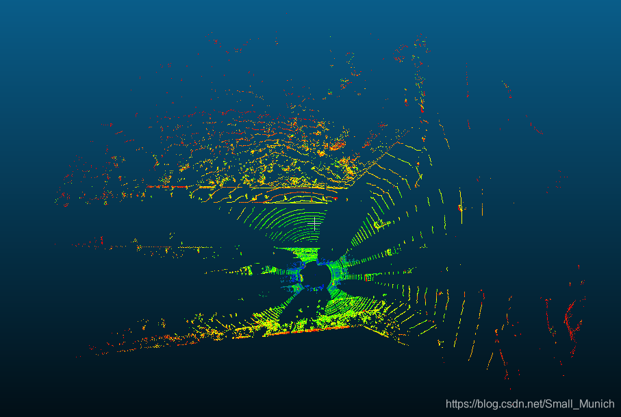
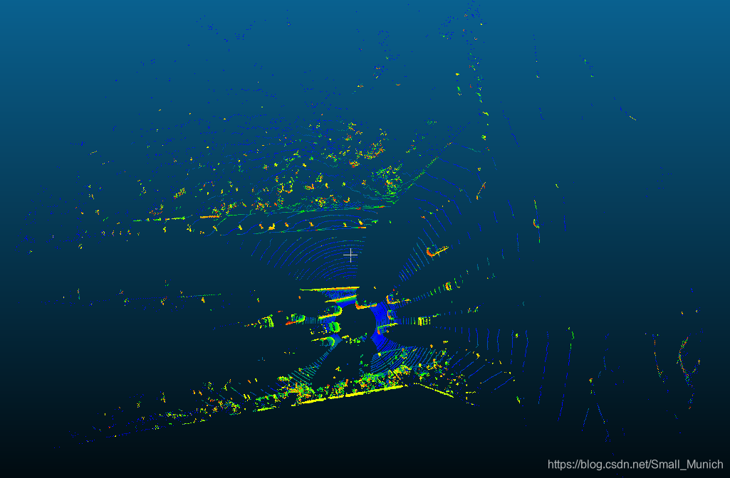
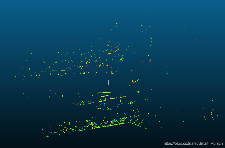
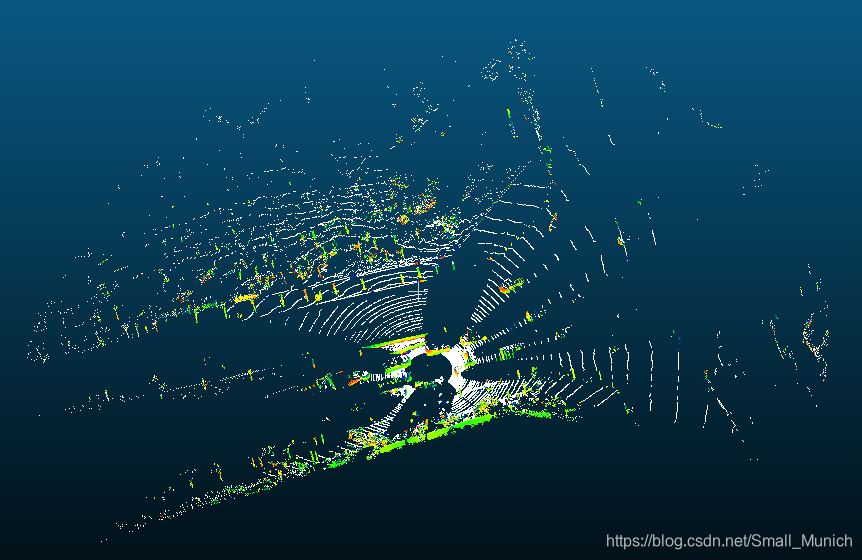
Demo实验结果可视化

Apollo原始点云 经过DoN法线差分后的点云 经过DoN法线差分按照阈值过滤后的点云 原始点云与滤波后点云叠加效果(白色可认为地面点)

论文中作者进行分割参数阈值的经验：

类别	$r_s$	$r_l$	$\Delta \hat{n}$
行人	0.1	0.4	$\frac{r_l}{r_s}\approx 10$
车辆	0.4	2.0	$\frac{r_l}{r_s}\approx 10$

　　论文中在滤波阶段丢弃$|\Delta \hat{n}|\le 0.25$的点云法线差分阈值，保留剩余下来的点云。由上图可视化可以看到，尺度较小时能够保留下道路中的边缘信息，随着尺度加大，只能够留下来具有较大的结构。这与图像中尺度空间原理一致。

　　消除不同尺度下法线差异由于方向估计模棱两可的情况：

小结

　　DoN(法线差异)求取方式思想主要来源于DoG(差分高斯)，我们都了解图像邻域DoG的应用多么有效，大名鼎鼎的SIFT算法就是采用DoG来提取图像特征。所有DoN在三维点云应用中，主要在有方向的3D边缘检测、平面区域分割等领域应用较好。很容易理解DoN主要也是在寻找三维空间中的显著性特征，就像图像领域中的梯度变化类似。但是，我们可以发现将法线差分的方式应用到地面点提取时候，会存在一些高程较高的平面被滤除掉，例如作者论文中的房屋结构信息等。另外，该方法耗时比较大，参数对于尺度较为敏感，不同的尺度参数分割出来差距会比较明显。同时该算法应用在离线点云处理可以，实时性地面分割无法有效保证使用。

参考

https://pcl-tutorials.readthedocs.io/en/latest/don_segmentation.html#don-segmentation