


💥💥💞💞欢迎来到本博客❤️❤️💥💥
🏆博主优势:🌞🌞🌞博客内容尽量做到思维缜密,逻辑清晰,为了方便读者。
⛳️座右铭:行百里者,半于九十。
📋📋📋本文目录如下:🎁🎁🎁
目录
⛳️赠与读者
👨💻做科研,涉及到一个深在的思想系统,需要科研者逻辑缜密,踏实认真,但是不能只是努力,很多时候借力比努力更重要,然后还要有仰望星空的创新点和启发点。建议读者按目录次序逐一浏览,免得骤然跌入幽暗的迷宫找不到来时的路,它不足为你揭示全部问题的答案,但若能解答你胸中升起的一朵朵疑云,也未尝不会酿成晚霞斑斓的别一番景致,万一它给你带来了一场精神世界的苦雨,那就借机洗刷一下原来存放在那儿的“躺平”上的尘埃吧。
或许,雨过云收,神驰的天地更清朗.......🔎🔎🔎
💥1 概述
雷达模拟测量及数字信号处理(DSP)检测目标研究
一、引言
雷达模拟测量是一种通过发射无线电波并接收其反射信号来检测目标物体的技术。随着计算机和通信技术的快速发展,数字信号处理(DSP)技术在雷达信号处理中得到了广泛应用。本文将详细介绍雷达模拟测量的基本原理,以及频率调制连续波(FMCW)波形生成、快速傅里叶变换(FFT)、距离-多普勒图和恒虚警率(CFAR)可视化等关键技术和方法。
二、雷达模拟测量基本原理
雷达测距的原理是利用电磁波的传播时间来计算目标物体与雷达之间的距离。当雷达向目标物体发送脉冲信号时,该信号会被物体反射回来并被雷达接收。通过测量发送信号和接收信号之间的时间差,可以得到目标物体与雷达之间的距离。
三、关键技术和方法
1. 频率调制连续波(FMCW)波形生成
FMCW雷达通过频率连续变化的波形发送和接收信号,以测量目标的距离。发送的信号频率在一段时间内缓慢变化,接收到的回波信号则与发送信号相比存在频率偏移。通过测量频率偏移,可以计算目标到雷达的距离。
2. 数字信号处理(DSP)
雷达接收到的回波信号是连续的模拟信号,需要使用数字信号处理技术来对其进行处理和分析。DSP技术包括滤波、采样、放大、频谱分析等一系列算法,用于提取目标的信息。在雷达信号处理中,DSP技术可以高速完成FFT、FIR、复数乘加以及矩阵运算等数字信号处理,从而提高信号的稳定性和抗干扰能力。
3. 快速傅里叶变换(FFT)
FFT是一种将时域信号转换为频域信号的算法。在雷达测量中,通过对接收到的信号进行FFT处理,可以得到信号的频谱信息,从而分析目标的速度信息。使用FFT算法进行雷达测距需要进行一系列的信号处理步骤,包括采样和数字化处理、FFT变换、频域数据分析等。FFT的应用不仅能够提高信号处理的速度和效率,还能够增强信号的抗干扰能力。
4. 距离-多普勒图
距离-多普勒图是一种将距离和速度信息可视化的方法。它将雷达接收到的信号进行距离和速度的双向处理,然后将结果以图像的形式显示出来,从而可以直观地观察目标的位置和速度信息。在绘制距离-多普勒图时,通常需要在距离维进行匹配滤波,以提高分辨能力;在多普勒维进行FFT,以提取多普勒频率。
5. 恒虚警率(CFAR)可视化
CFAR是一种用于雷达信号处理的算法,在背景杂波较大的情况下,可以实现目标的自适应检测。CFAR根据背景杂波的统计特性,动态调整检测阈值,以保持恒定的虚警率,并有效地检测目标信号。通过CFAR可视化,可以直观地观察到目标信号在背景杂波中的存在情况,从而提高目标检测的准确性。
四、研究方法和步骤
- FMCW波形生成:通过改变频率的连续波形来实现测量,生成FMCW信号。
- 信号接收与处理:接收雷达回波信号,并进行数字信号处理(DSP),包括滤波、采样、放大等步骤。
- FFT变换:对处理后的信号进行快速傅里叶变换(FFT),得到频域上的信号数据。
- 距离-多普勒图绘制:根据FFT变换结果,绘制距离-多普勒图,显示目标的位置和速度信息。
- CFAR可视化:应用CFAR算法对距离-多普勒图进行处理,实现目标的自适应检测,并进行可视化展示。
五、结论与展望
本文通过介绍频率调制连续波(FMCW)波形生成、快速傅里叶变换(FFT)、距离-多普勒图和恒虚警率(CFAR)可视化等关键技术和方法,详细阐述了雷达模拟测量及数字信号处理(DSP)检测目标的基本原理和步骤。这些技术和方法的结合使用,可以实现对目标的准确检测和定位,并通过可视化的方式直观地观察目标的位置和速度信息。未来,随着计算机和通信技术的不断发展,雷达模拟测量和数字信号处理技术将在更多领域得到广泛应用,为相关领域的发展做出更大贡献。
📚2 运行结果

部分代码:
%% Target Position & Velocity
% initial position/ range
d0 = 80;
% velocity (assumed constant)
v0 = -50;
%% FMCW Waveform Design
d_res = 1;
speed_of_light = 3*10^8; % 3e8
RMax = 200;
Bsweep = speed_of_light / (2 * d_res); % bandwidth
Tchirp = 5.5 * 2 * RMax / speed_of_light; % chirp time
alpha = Bsweep / Tchirp; % slope of FMCW chirps
fc = 77e9; % carrier frequency of radar
Nd = 128; % number of chirps in one sequence
Nr = 1024; % number of samples on each chirp
t = linspace(0, Nd * Tchirp, Nr * Nd); % total time for samples
% vectors for Tx, Rx and Mix based on the total samples input
Tx = zeros(1, length(t)); % transmitted signal
Rx = zeros(1, length(t)); % received signal
Mix = zeros(1, length(t)); % beat signal
% vectors for range covered and time delay
r_t = zeros(1, length(t));
td = zeros(1, length(t));
%% Signal generation and Moving Target simulation
% Running the radar scenario over the time.
for i = 1:length(t)
% for each timestamp update the range of the target for constant velocity
r_t(i) = d0 + v0 * t(i);
td(i) = 2 * r_t(i) / speed_of_light;
% for each time sample update the transmitted and received signal
Tx(i) = cos(2 * pi * (fc * t(i) + alpha * t(i)^2 / 2));
Rx(i) = cos(2 * pi * (fc * (t(i) - td(i)) + (alpha * (t(i) - td(i))^2) / 2));
% now by mixing the transmit and receive generate the beat signal by performing
% element-wise matrix multiplication of transmit and receiver signal
Mix(i) = Tx(i) .* Rx(i); % beat signal
end
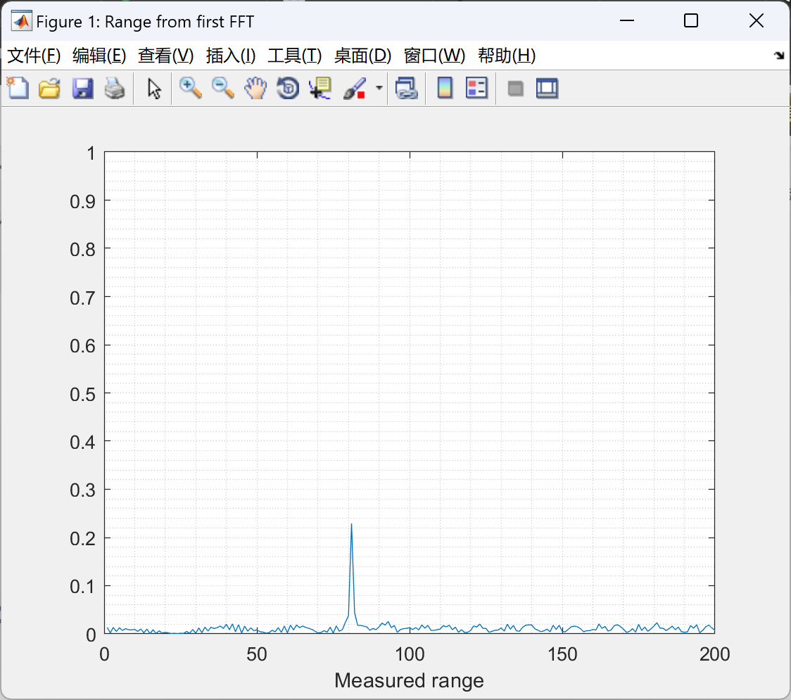
%% RANGE MEASUREMENT
% reshaping vector into Nr*Nd array. Nr and Nd here also define the size of range and doppler FFT respectively
% running the Fast Fourier Transform (FFT) on the beat signal along the range bins dimension (Nr) and normalise
sig_fft = fft(Mix, Nr) ./ Nr;
% taking absolute value of FFT output
sig_fft = abs(sig_fft);
% output of FFT is double-sided signal, but since we are interested in one side of the spectrum only, we throw out half of the samples
sig_fft = sig_fft(1 : (Nr / 2));
figure('Name', 'Range from first FFT') % plot range
plot(sig_fft); grid minor % plot FFT output
axis([0 200 0 1]);
xlabel('Measured range');
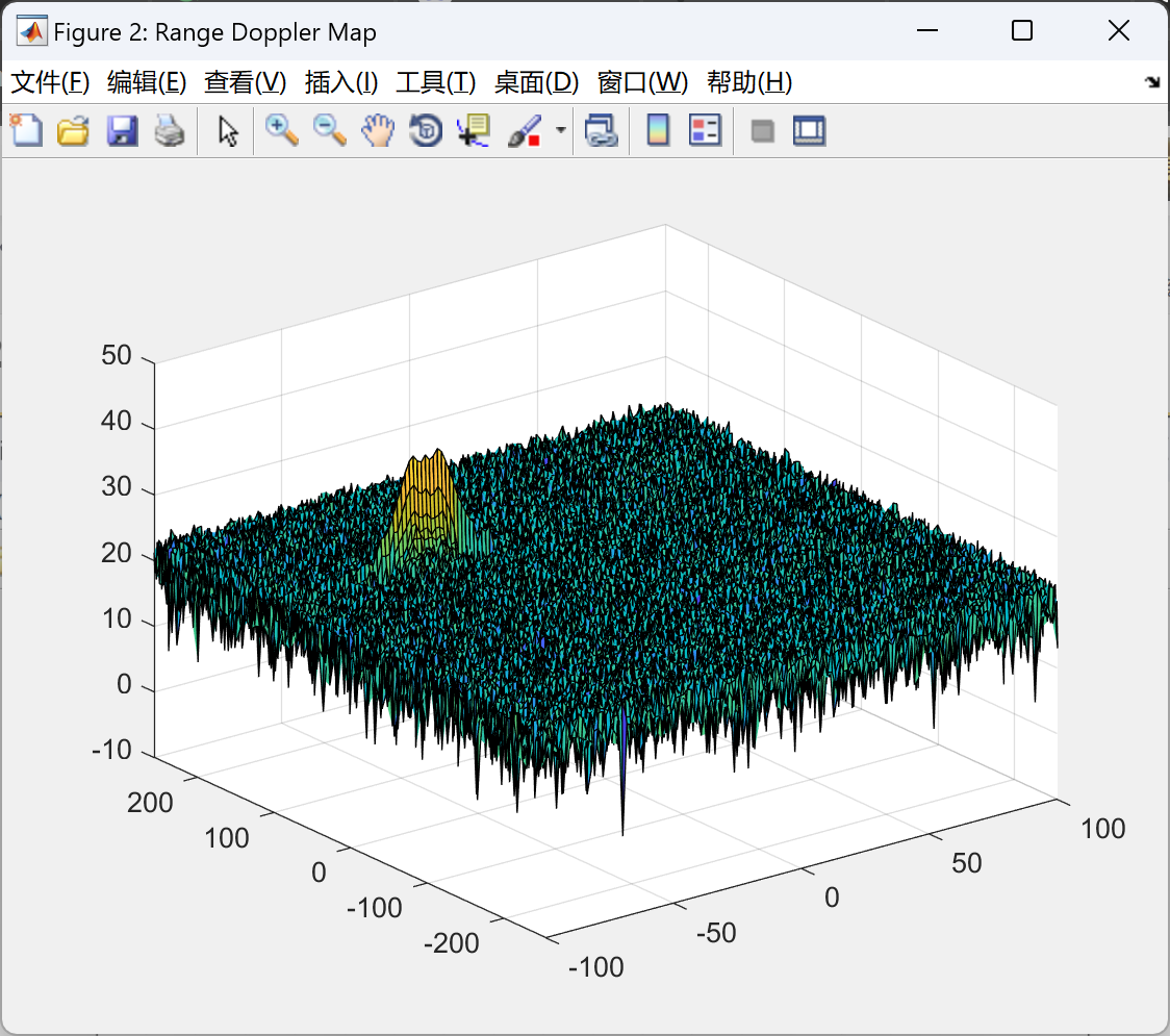
%% RANGE DOPPLER RESPONSE
% Running a 2D FFT on the mixed signal (beat signal) output and generate a Range Doppler Map (RDM)
% The output of the 2D FFT is an image that has reponse in the range and doppler FFT bins.
% Therefore, it is important to convert the axis from bin sizes to range and doppler based on their max values
Mix = reshape(Mix, [Nr, Nd]);
% 2D FFT using the FFT size for both dimensions
sig_fft2 = fft2(Mix, Nr, Nd);
% taking just one side of signal from range dimension
sig_fft2 = sig_fft2(1 : Nr / 2, 1 : Nd);
sig_fft2 = fftshift(sig_fft2);
RDM = abs(sig_fft2);
RDM = 10*log10(RDM);
% use surf function to plot output of 2D-FFT and show axis in both dimensions
doppler_axis = linspace(-100, 100, Nd);
range_axis = linspace(-200, 200, Nr/2) * ((Nr / 2) / 400);
figure('Name', 'Range Doppler Map'), surf(doppler_axis, range_axis, RDM);
%% CFAR Implementation
% sliding window through the complete Range Doppler Map (RDM)
% selecting number of training cells in both the dimensions
Tcr = 10;
Tcd = 4;
% selecting number of guard cells in both dimensions around the Cell Under Test (CUT) for accurate estimation
Gcr = 5;
Gcd = 2;
% offsetting the threshold by signal-to-noise-ratio (SNR) value in dB
offset = 1.4;
% creating vector to store noise level for each iteration on training cells
noise_level = zeros(Nr / 2 - 2 * (Tcd + Gcd), Nd - 2 * (Tcr + Gcr));
gridSize = (2 * Tcr + 2 * Gcr + 1) * (2 * Tcd + 2 * Gcd + 1);
trainingCellsNum = gridSize - (2 * Gcr + 1) * (2 * Gcd + 1);
% designing loop - slide the CUT across range doppler map by giving margins
% at the edges for training and guard cells.
% For every iteration sum the signal level within all the training cells
% To sum convert the value from logarithmic to linear using db2pow function
% Average the summed values for all of the training cells used
% After averaging, convert it back to logarithimic using pow2db
% Add the offset to it to determine the threshold
% Next, compare the signal under CUT with this threshold:
% if the CUT level > threshold, assign it a value of 1, else equate it to 0
CFAR_sig = zeros(size(RDM));
% Using RDM[x,y] as the matrix from the output of 2D FFT for implementing CFAR
for j = 1 : Nd - 2 * (Tcr + Gcr)
for i = 1 : Nr / 2 - 2 * (Tcd + Gcd)
% to extract only the training cells, first get the sliding patch and,
% after converting it to power from decibel, set to zero whatever isn't
% in the position of training cells;
% the zero submatrix will not contribute to the sum over the whole patch and,
% by dividing for the number of training cells I will get the noise mean level
trainingCellsPatch = db2pow(RDM( i : i + 2 * (Tcd + Gcd), j : j + 2 * (Gcr + Tcr)));
trainingCellsPatch(Tcd + 1 : end - Tcd, Tcr + 1 : end - Tcr) = 0;
noise_level(i,j) = pow2db(sum(sum(trainingCellsPatch))/trainingCellsNum);
sigThresh = noise_level(i, j) * offset;
if RDM(i + (Tcd + Gcd), j + (Tcd + Gcr)) > sigThresh
CFAR_sig(i + (Tcd + Gcd), j + (Tcd + Gcr)) = 1;
else
CFAR_sig(i + (Tcd + Gcd), j + (Tcd + Gcr)) = 0;
end
end
🎉3 参考文献
文章中一些内容引自网络,会注明出处或引用为参考文献,难免有未尽之处,如有不妥,请随时联系删除。(文章内容仅供参考,具体效果以运行结果为准)
[1]李菊,陈禾,金俊坤,等.基于FFT的两种伪码快速捕获方案的研究与实现[J].电子与信息学报, 2006.
[2]姬红兵.一种基于数字信号处理器的有效FFT实现[J].西安电子科技大学学报, 1998, 25(4):5.
[3]郑慧.基于离散傅里叶变换的电网谐波测量方法与分析研究[D].上海海事大学,2006.
🌈4 Matlab代码实现
资料获取,更多粉丝福利,MATLAB|Simulink|Python资源获取


 1081
1081

 被折叠的 条评论
为什么被折叠?
被折叠的 条评论
为什么被折叠?
 到【灌水乐园】发言


