


写在前面
WGCNA的教程,我们在前期的推文中已经退出好久了。今天在结合前期的教程的进行优化一下。只是在现有的教程基础上,进行修改。其他的其他并无改变。
前期WGCNA教程
本次教程的优化点
注意:本次教程在教程二的基础上修改。
- 教程代码更规范
- 教程添加了过滤数值流程
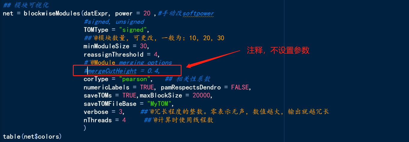
- 教程添加merge模块后图形绘制(注:在教程二的基础上)
- 教程添加更多的注释信息
- 教程后期添加视频讲解
WGCNA教程 | 代码四
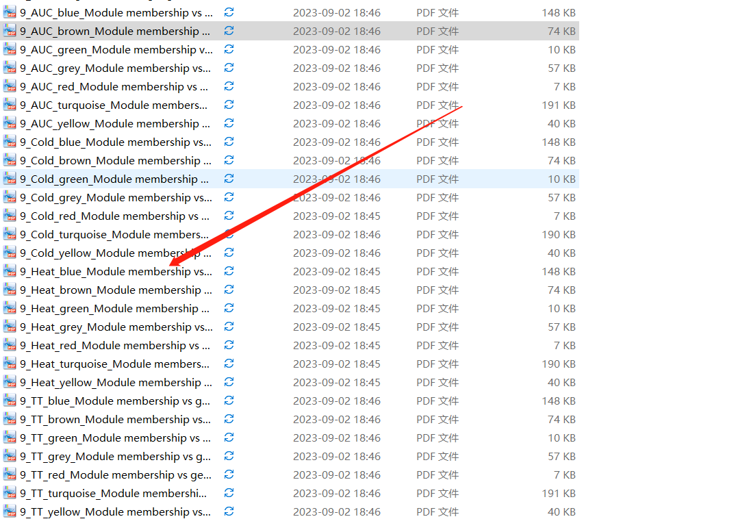
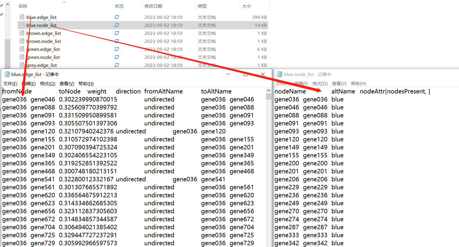
本期教程输出所有的文件信息。
设置文件位置及导入包
##'@加权基因共表达分析(WGCNA)
##'@2023.09.02
##'@整理者:小杜的生信笔记
##'@前期教程网址:https://mp.weixin.qq.com/s/Ln9TP74nzWhtvt7obaMp1A
##'
##'@本教程主要主要是为了优化前期代码,在前期的基础上进行修改。
##'@若您的数据量较大,我们建议WGCNA在服务器上跑。
##'

##==============================================================================

setwd("E:\\小杜的生信筆記\\2023\\20230217_WGCNA\\WGCNA_04")
rm(list = ls())
#install.packages("WGCNA")
#BiocManager::install('WGCNA')
library(WGCNA)
options(stringsAsFactors = FALSE)
#enableWGCNAThreads(60) ## 打开多线程
#Read in the female liver data set
导入数据
我们这里给出了两种不同文件的导入方式,txt和csv。
#'@导入数据
#'@导入txt格式数据
# WGCNA.fpkm = read.table("ExpData_WGCNA.txt",header=T,
#                         comment.char = "",
#                         check.names=F)
##'@导入csv文件格式
WGCNA.fpkm = read.csv("ExpData_WGCNA.csv", header = T, check.names = F)
WGCNA.fpkm[1:10,1:10]
检查数据缺失值
gsg = goodSamplesGenes(datExpr0, verbose = 3)
gsg$allOK
if (!gsg$allOK)
{
  if (sum(!gsg$goodGenes)>0)
    printFlush(paste("Removing genes:", paste(names(datExpr0)[!gsg$goodGenes], collapse = ", ")))
  if (sum(!gsg$goodSamples)>0)
    printFlush(paste("Removing samples:", paste(rownames(datExpr0)[!gsg$goodSamples], collapse = ", ")))
  # Remove the offending genes and samples from the data:
  datExpr0 = datExpr0[gsg$goodSamples, gsg$goodGenes]
}
过滤数值 [optional]
@过滤数值(optional),此步根据你自己的数据进行过滤数值,过滤的数值大小根据自己需求修改
meanFPKM=0.5  ###--过滤标准,可以修改
n=nrow(datExpr0)
datExpr0[n+1,]=apply(datExpr0[c(1:nrow(datExpr0)),],2,mean)
datExpr0=datExpr0[1:n,datExpr0[n+1,] > meanFPKM]
# for meanFpkm in row n+1 and it must be above what you set--select meanFpkm>opt$meanFpkm(by rp)
filtered_fpkm=t(datExpr0)
filtered_fpkm=data.frame(rownames(filtered_fpkm),filtered_fpkm)
names(filtered_fpkm)[1]="sample"
head(filtered_fpkm)
###'@输出过滤的文件
write.table(filtered_fpkm, file="WGCNA.filter.txt",
            row.names=F, col.names=T,quote=FALSE,sep="\t")
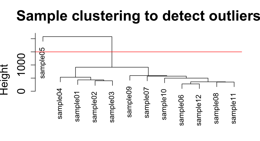
样本聚类
###'@样本聚类
sampleTree = hclust(dist(datExpr0), method = "average")
pdf("1_sample clutering.pdf", width = 6, height = 4)
par(cex = 0.7);
par(mar = c(0,4,2,0))
plot(sampleTree, main = "Sample clustering to detect outliers", sub="", xlab="", cex.lab = 1.5,
     cex.axis = 1.5, cex.main = 2)
dev.off()

样本sample05与整体数据差异较大,过滤此数据。
过滤样本
pdf("2_sample clutering_delete_outliers.pdf", width = 6, height = 4)
plot(sampleTree, main = "Sample clustering to detect outliers", sub="", xlab="", cex.lab = 1.5,
cex.axis = 1.5, cex.main = 2) +
abline(h = 1500, col = "red") ###'@"h = 1500"参数为你需要过滤的参数高度
dev.off()
##'@过滤离散样本
##'@"cutHeight"为过滤参数,与上述图保持一致
clust = cutreeStatic(sampleTree, cutHeight = 1500, minSize = 10)
keepSamples = (clust==1)
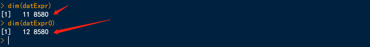
datExpr = datExpr0[keepSamples, ]
nGenes = ncol(datExpr)
nSamples = nrow(datExpr)
两个样本直接数据比较
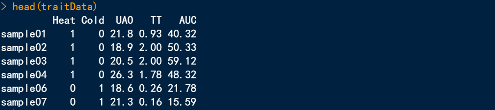
载入性状数据
##'@导入csv格式
traitData = read.csv("TraitData.csv",row.names=1)
# ##'@导入txt格式
# traitData = read.table("TraitData.txt",row.names=1,header=T,comment.char = "",check.names=F)
head(traitData)
allTraits = traitData
dim(allTraits)
names(allTraits)
# 形成一个类似于表达数据的数据框架
fpkmSamples = rownames(datExpr)
traitSamples =rownames(allTraits)
traitRows = match(fpkmSamples, traitSamples)
datTraits = allTraits[traitRows,]
rownames(datTraits)
collectGarbage()
Re-cluster samples
# Re-cluster samples
sampleTree2 = hclust(dist(datExpr), method = "average")
#
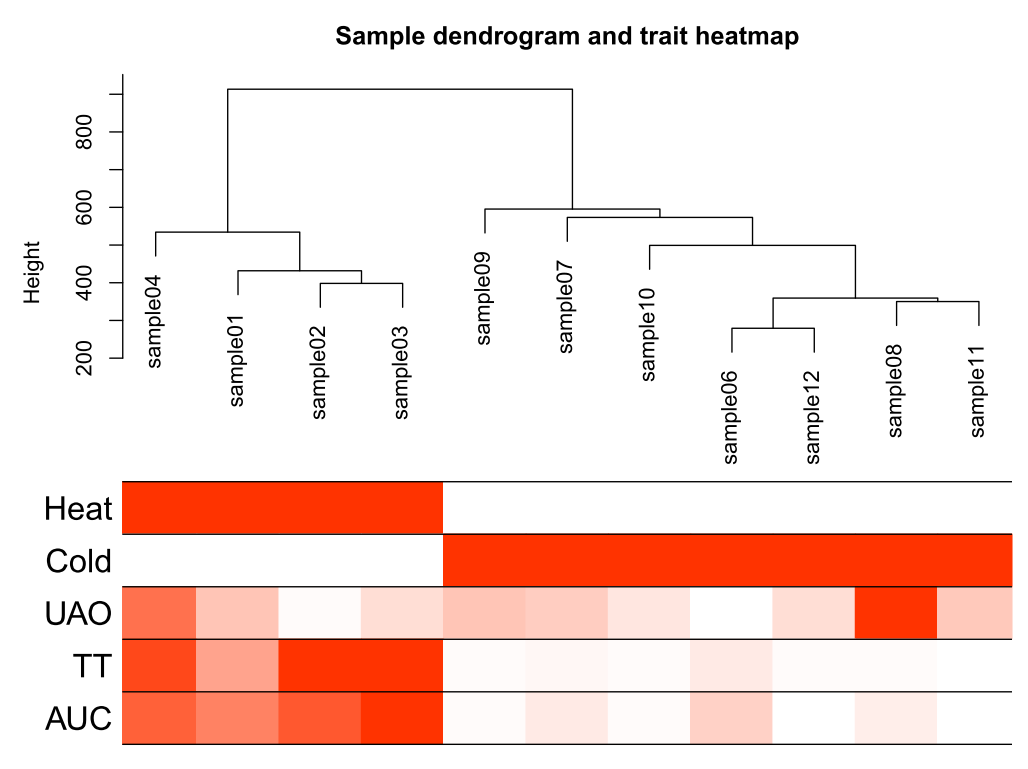
traitColors = numbers2colors(datTraits, signed = FALSE)
# Plot the sample dendrogram and the colors underneath.
Sample dendrogram and trait heatmap
#sizeGrWindow(12,12)
pdf(file="3_Sample_dendrogram_and_trait_heatmap.pdf",width=8 ,height= 6)
plotDendroAndColors(sampleTree2, traitColors,
                    groupLabels = names(datTraits),
                    main = "Sample dendrogram and trait heatmap",cex.colorLabels = 1.5, cex.dendroLabels = 1, cex.rowText = 2)
dev.off()
数据处理结束,继续后续网络构建分析!
#'@打开多线程分析
enableWGCNAThreads(5)
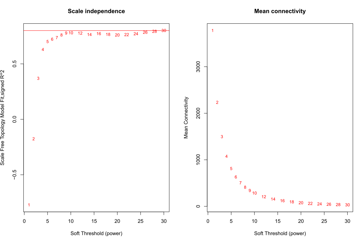
获得最佳阈值(softpower)
#'@获得soft阈值
#powers = c(1:30)
powers = c(c(1:10), seq(from = 12, to=30, by=2))
#'@调用网络拓扑分析功能
sft = pickSoftThreshold(datExpr, powerVector = powers, verbose = 5)
绘制softpower图形
#'@绘制soft power plot
pdf(file="4_软阈值选择.pdf",width=12, height = 8)
par(mfrow = c(1,2))
cex1 = 0.85
# Scale-free topology fit index as a function of the soft-thresholding power
plot(sft$fitIndices[,1], -sign(sft$fitIndices[,3])*sft$fitIndices[,2],
     xlab="Soft Threshold (power)",ylab="Scale Free Topology Model Fit,signed R^2",type="n",
     main = paste("Scale independence"));
text(sft$fitIndices[,1], -sign(sft$fitIndices[,3])*sft$fitIndices[,2],
     labels=powers,cex=cex1,col="red");
# this line corresponds to using an R^2 cut-off of h
abline(h=0.8,col="red")
# Mean connectivity as a function of the soft-thresholding power
plot(sft$fitIndices[,1], sft$fitIndices[,5],
     xlab="Soft Threshold (power)",ylab="Mean Connectivity", type="n",
     main = paste("Mean connectivity"))
text(sft$fitIndices[,1], sft$fitIndices[,5], labels=powers, cex=cex1,col="red")
dev.off()
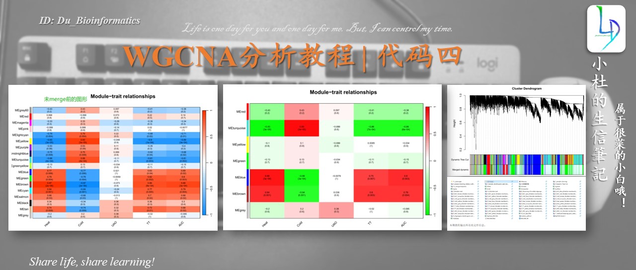
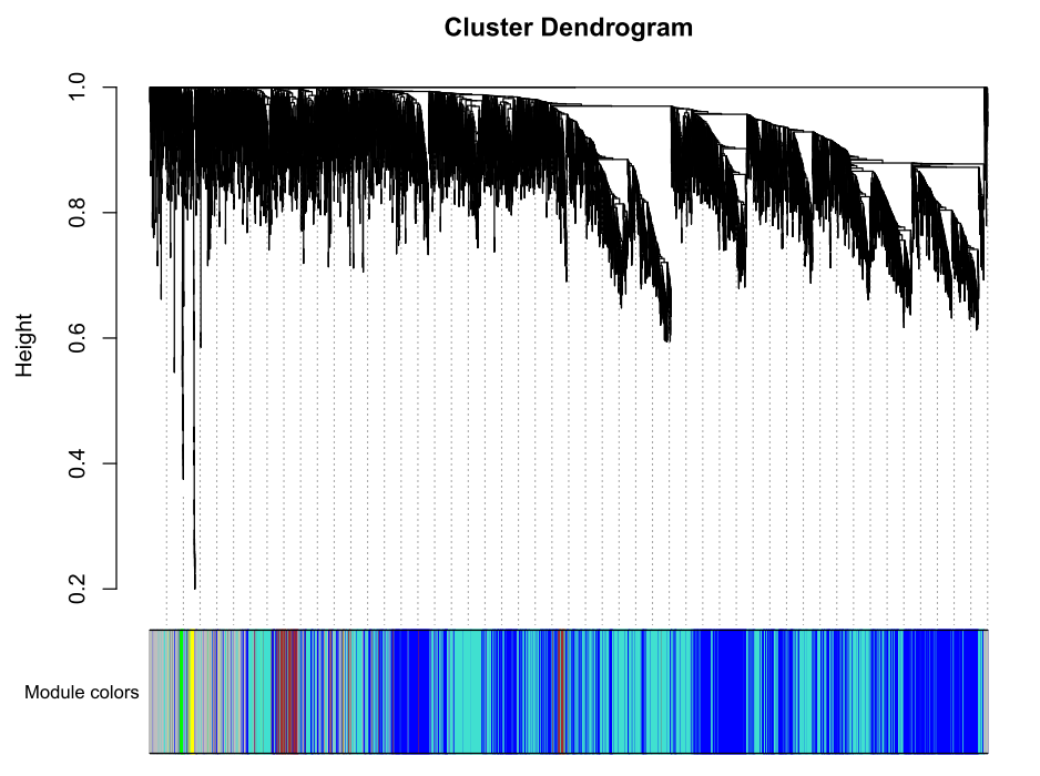
详细教程请看:WGCNA分析教程 | 代码四
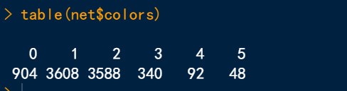

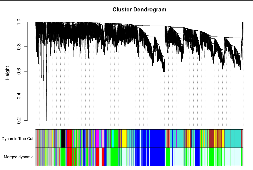
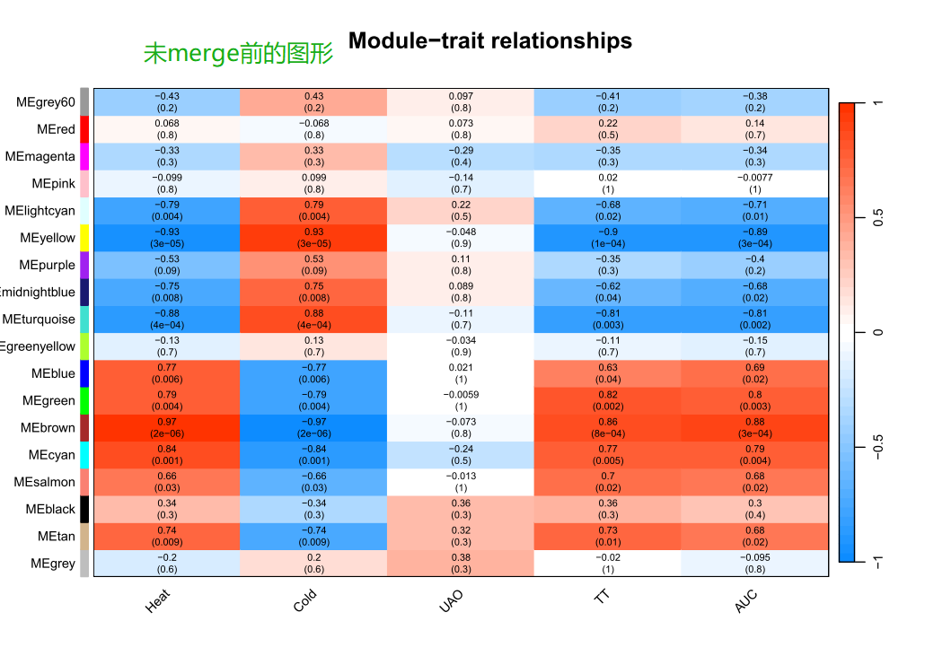
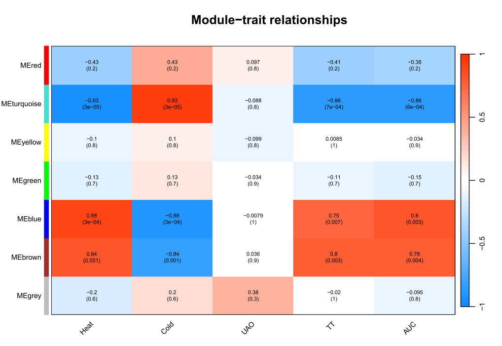
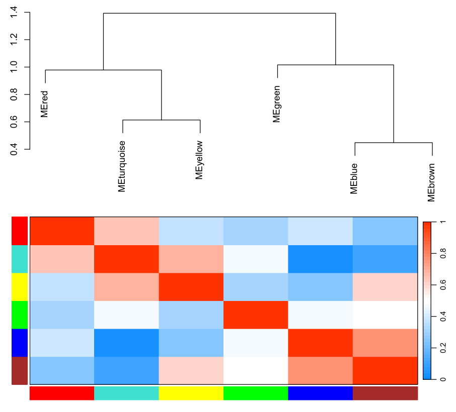
merge后的图形【我们最终获得图形】

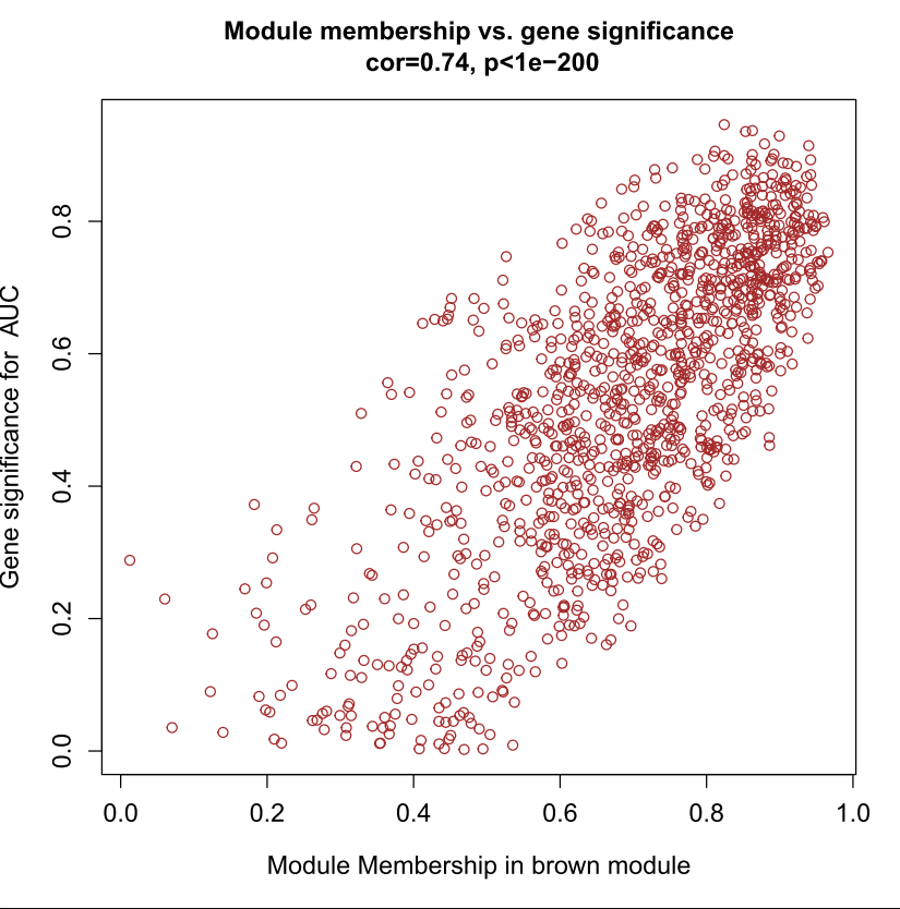
输出模块与基因相关性散点图
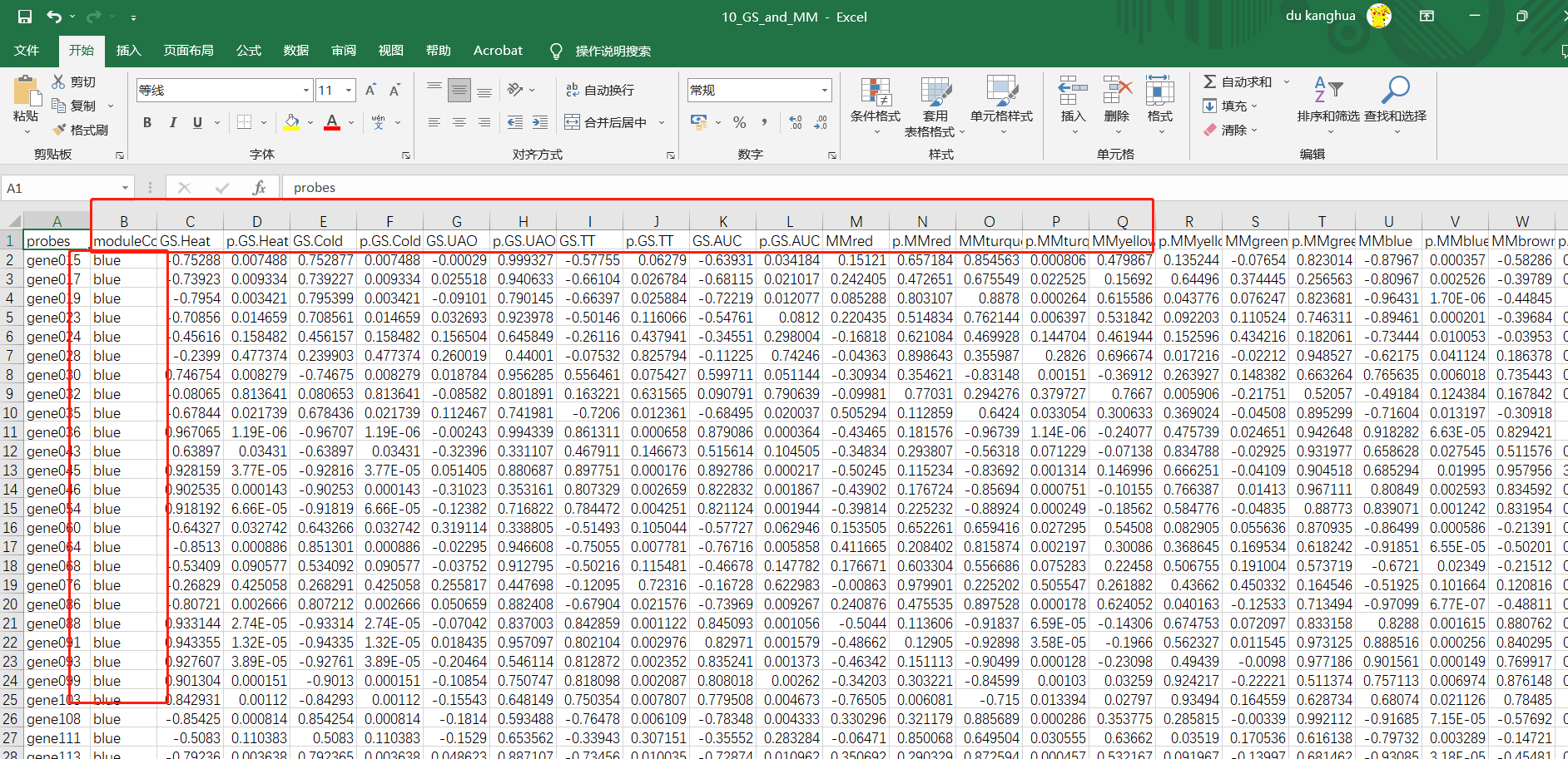
输出MM和GS数据
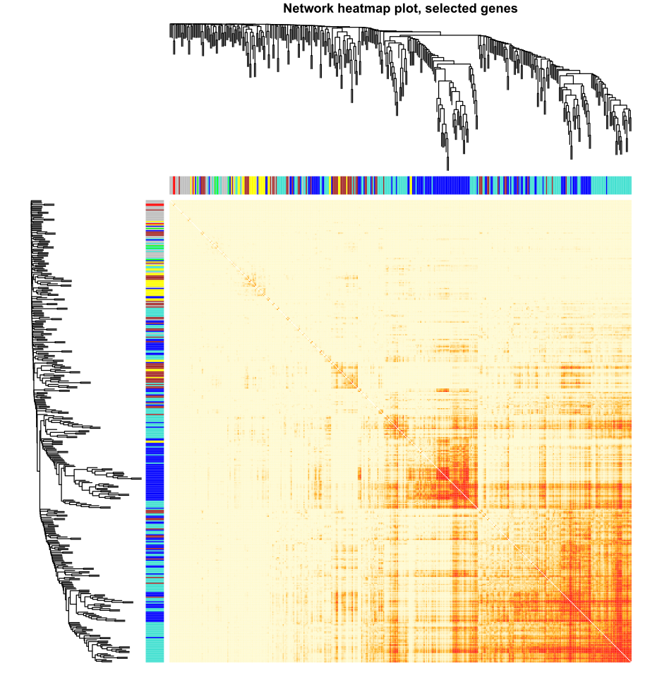
Network heatmap plot
小杜的生信筆記,主要发表或收录生物信息学的教程,以及基于R的分析和可视化(包括数据分析,图形绘制等);分享感兴趣的文献和学习资料!!


 837
837


 被折叠的 条评论
为什么被折叠?
被折叠的 条评论
为什么被折叠?
 到【灌水乐园】发言


