知识分享| 转录组个性化分析(6）——WGCNA

       近年来，很多SCI高分文章中都使用了WGCNA，那么WGCNA是什么，它可以应用于哪些研究方向，又如何进行WGCNA分析，其分析结果如何看？现在就带着这些问题，跟着小易一起学习探讨吧！

1  WGCNA介绍

       WGCNA（weighted gene co-expression network analysis，权重基因共表达网络分析）是一种分析多个样本基因表达模式的分析方法，可将表达模式相似的基因进行聚类，并分析模块与特定性状或表型之间的关联关系，因此在疾病以及其他性状与基因关联分析等方面的研究中被广泛应用。

WGCNA与趋势分析都为基因共表达分析方法，与趋势分析相比，WGCNA 有以下优势：

a. 聚类方法：使用权重共表达策略（无尺度分布），更加符合生物学现象；

b. 基因间的关系：能呈现基因间的相互作用关系，且能找出处于调控网络中心的 hub 基因；

c. 样本数：适合于大样本量，且越多越好。而趋势分析 5 个点以上就会使结果非常复杂，准确性 下降，且最多只能分析 8 个点；

d. 与表型的关联：可以利用模块特征值和 hub 基因与特定性状、表型进行关联分析，更准确地分 析生物学问题。

2  数据要求

       由于WGCNA是基于相关系数的表达调控网络分析方法。当样本数过低的时候，相关系数的计算是不可靠的，得到的调控网络价值不大。所以，我们推荐的样本数如下：

a. 当独立样本数≥8（非重复样本）时，可以考虑基于Pearson相关系数的WGCNA共表达网络的方法（效果看实际情况而定）；

b. 当样本数≥15（可以包含生物学重复）时，WGCNA方法会有更好的效果。

c. 当样品数＜8时，不建议进行该项分析。

d. 该方法对于不同材料或不同组织进行分析更有意义，对于不同时间点处理相同样品意义不大。

3  分析代码

a. wgcna01_1.R，wgcna01_2.R是用来构建网络和相关图，适用于性状关联和无性状关联的WGCNA网络构建。因为这两步很费时，就拆开了并行跑。

用法：Rscript wgcna01_1.R expre.xls;

b. wgcna02.R 是可视化基因网络图。

Rscript wgcna02.R trait.txt(optional)

代码：wgcna01_1

# Description: To perform co‐expression analysis based on WGCNA Rpackage
# Version: 1.0, mics.com, 2018‐10‐09
# Usage: Rscript wgcna.R rpkm.xls outdir
args <‐ commandArgs(TRUE);
exp_data=args[1]
# Part 1. Basic Analysis
# 1. Data input, cleaning and pre‐processing
# 1.1 Loading expression data
# Load the package
library(WGCNA);
# The following setting is important, do not omit.
options(stringsAsFactors = FALSE);
#Read in the data set
data = read.table(exp_data, head=T, row.names=1);
multiExpr = t(data);
# 1.2 Checking data for excessive missing values
gsg = goodSamplesGenes(multiExpr, verbose = 3);
#
if (!gsg$allOK)
{
# Remove the offending genes and samples from the data:
multiExpr = multiExpr[gsg$goodSamples, gsg$goodGenes]
}

nGenes = ncol(multiExpr)
nSamples = nrow(multiExpr)

if(nGenes > 30000)
{
library(genefilter)
data = read.table(exp_data, head=T, row.names=1)
f1 <‐ pOverA(0.8,0.5)
f2 <‐ function(x) (IQR(x) > 0.5)
ff <‐ filterfun(f1, f2)
selected <‐ genefilter(data, ff)
sum(selected)
esetSub <‐ data[selected, ]
multiExpr <‐ as.data.frame(t(esetSub))
nGenes = ncol(multiExpr)
nSamples = nrow(multiExpr)
}

save(multiExpr, file = "01‐dataInput_Expr.RData")

####Plot 1 samples cluster
sampleTree = hclust(dist(multiExpr), method = "average");
sizeGrWindow(12,9)
pdf(file = "sampleClustering.pdf", width = 12, height = 9);
par(cex = 0.6);
par(mar = c(0,4,2,0))
plot(sampleTree, main = "Sample clustering to detect outliers",
sub="", xlab="", cex.lab = 1.5,cex.axis = 1.5, cex.main = 2)
dev.off()

#########################################remove outlier samples(depend
on samples totally)
# Plot a line to show the cut
#abline(h = 15, col = "red");
# Determine cluster under the line
#clust = cutreeStatic(sampleTree, cutHeight = 15, minSize = 10)
#table(clust)
# clust 1 contains the samples we want to keep.
#keepSamples = (clust==1)
#multiExpr = multiExpr[keepSamples, ]
#nGenes = ncol(multiExpr)
#nSamples = nrow(multiExpr)
# 2. Step‐by‐step network construction and module detection
#=====================================================================
=========
# 2.1 Choosing the soft‐thresholding power: analysis of network
# Choose a set of soft‐thresholding powers
powers = c(c(1:10), seq(from = 12, to=30, by=2))
# Call the network topology analysis function
sft = pickSoftThreshold(multiExpr, powerVector = powers, verbose = 5 )
save(sft, file = "01‐sftpower.RData")

####Plot 2 selected power
pdf(file ="Network_power.pdf", width = 9, height = 5);
par(mfrow = c(1,2));
cex1 = 0.9;
# Scale‐free topology fit index as a function of the soft‐thresholdingpower
plot(sft$fitIndices[,1], ‐sign(sft$fitIndices[,3])*sft$fitIndices[,2],
xlab="Soft Threshold (power)",ylab="Scale Free Topology ModelFit,signed R^2",type="n",
main = paste("Scale independence"));
text(sft$fitIndices[,1], ‐sign(sft$fitIndices[,3])*sft$fitIndices[,2],
labels=powers,cex=cex1,col="red");
abline(h=0.85,col="red")
# Mean connectivity as a function of the soft‐thresholding power
plot(sft$fitIndices[,1], sft$fitIndices[,5],
xlab="Soft Threshold (power)",ylab="Mean Connectivity", type="n",
main = paste("Mean connectivity"))
text(sft$fitIndices[,1], sft$fitIndices[,5], labels=powers,
cex=cex1,col="red")
dev.off()
# Select power
softPower <‐ sft$powerEstimate
####Plot 3 检验选定的β值下记忆网络是否逼近 scale free
# 基因多的时候使用下面的代码:
k <‐ softConnectivity(datE=multiExpr,power=softPower)
pdf(file = "Check_Scalefree.pdf", width = 10, height = 5);
par(mfrow=c(1,2))
hist(k)
scaleFreePlot(k,main="Check Scale free topology\n")
#‐‐‐‐‐‐‐‐‐‐‐‐‐‐‐‐‐‐‐‐‐‐‐‐‐‐‐‐‐‐‐‐‐‐‐‐‐‐‐‐‐‐‐‐‐‐‐‐‐‐‐‐‐‐‐‐‐‐‐‐‐‐‐‐‐‐‐‐‐
‐‐‐‐‐‐‐‐‐
# 2.2 One‐step network construction and module detection
#‐‐‐‐‐‐‐‐‐‐‐‐‐‐‐‐‐‐‐‐‐‐‐‐‐‐‐‐‐‐‐‐‐‐‐‐‐‐‐‐‐‐‐‐‐‐‐‐‐‐‐‐‐‐‐‐‐‐‐‐‐‐‐‐‐‐‐‐‐
‐‐‐‐‐‐‐‐‐
#2.2.1 获得临近矩阵,根据β值获得临近矩阵和拓扑矩阵，：
softPower <‐ sft$powerEstimate
adjacency = adjacency(multiExpr, power = softPower);
# 将临近矩阵转为 Tom 矩阵
TOM = TOMsimilarity(adjacency);
# 计算基因之间的相异度
dissTOM = 1‐TOM
save(TOM, file = "TOMsimilarity_adjacency.RData")
#2.2.2a Clustering using TOM
geneTree = hclust(as.dist(dissTOM),method="average");
minModuleSize = 30
dynamicMods = cutreeDynamic(dendro = geneTree, distM = dissTOM,
minClusterSize = minModuleSize);
table(dynamicMods)
dynamicColors = labels2colors(dynamicMods)
table(dynamicColors)
#Plot 4 plot the dendrogram and colors underneath
pdf(file = "GeneDendrogramColors.pdf", width = 12, height = 9);
sizeGrWindow(12,9)
plotDendroAndColors(geneTree, dynamicColors,
"Dynamic Tree Cut",
dendroLabels = FALSE, hang = 0.03,
addGuide = TRUE, guideHang = 0.05,
main = "Gene dendrogram and module colors")
dev.off()
#2.2.2b Merging of modules whose expression profiles are very similar
MEList = moduleEigengenes(multiExpr, colors = dynamicColors)
MEs = MEList$eigengenes
MEDiss = 1‐cor(MEs);
METree = hclust(as.dist(MEDiss), method = "average");
#Plot 5 merge the dendrogram and colors underneath for similar module
pdf(file = "Clustering_similar_module.pdf", width = 12, height = 9);
sizeGrWindow(12, 9)
plot(METree, main = "Clustering of similar module eigengenes",
xlab = "", sub = "")
MEDissThres = 0.25
abline(h=MEDissThres, col = "red")
dev.off()
merge = mergeCloseModules(multiExpr, dynamicColors, cutHeight =
MEDissThres, verbose = 3)
mergedColors = merge$colors;
mergedMEs = merge$newMEs;
#Plot 6 plot the gene dendrogram again, with the original and merged
module colors underneath
pdf(file = "Merged_GeneDendrogramColors.pdf", width = 12, height = 9)
sizeGrWindow(12, 9)
plotDendroAndColors(geneTree, cbind(dynamicColors, mergedColors), c("Dynamic Tree Cut", "Merged dynamic"),
dendroLabels = FALSE, hang = 0.03, addGuide = TRUE, guideHang = 0.05)
dev.off()
moduleColors = mergedColors
colorOrder = c("grey", standardColors(50));
moduleLabels = match(moduleColors, colorOrder)‐1;
MEs = mergedMEs;
save(MEs, moduleLabels, moduleColors, geneTree, file = "02‐networkConstruction‐stepByStep.RData")

 代码：wgcna01_2

args <‐ commandArgs(TRUE);
exp_data=args[1]
# Part 1.1 Tom Network visualization
# 1. Data input, cleaning and pre‐processing
# 1.1 Loading expression data
# Load the package
library(WGCNA);
options(stringsAsFactors = FALSE)
enableWGCNAThreads()
# The following setting is important, do not omit.
options(stringsAsFactors = FALSE);
#Read in the data set
data = read.table(exp_data, head=T, row.names=1);
multiExpr = t(data)
# 1.2 Checking data for excessive missing values
gsg = goodSamplesGenes(multiExpr, verbose = 3);
#
if (!gsg$allOK)
{
# Remove the offending genes and samples from the data:
multiExpr = multiExpr[gsg$goodSamples, gsg$goodGenes]
}
nGenes = ncol(multiExpr)
nSamples = nrow(multiExpr)
if(nGenes > 30000)
{
library(genefilter)
data = read.table(exp_data, head=T, row.names=1)
f1 <‐ pOverA(0.8,0.5)
f2 <‐ function(x) (IQR(x) > 0.5)
ff <‐ filterfun(f1, f2)
selected <‐ genefilter(data, ff)
sum(selected)
esetSub <‐ data[selected, ]
multiExpr <‐ as.data.frame(t(esetSub))
nGenes = ncol(multiExpr)
nSamples = nrow(multiExpr)
}
# 1.3 Choosing the soft‐thresholding power: analysis of network
topology
# Choose a set of soft‐thresholding powers
powers = c(c(1:10), seq(from = 12, to=30, by=2))
# Call the network topology analysis function
sft = pickSoftThreshold(multiExpr, powerVector = powers, verbose = 5 )
softPower <‐ sft$powerEstimate
# 1.4 Visualizing the gene network
# Calculate topological overlap anew: this could be done more
efficiently by saving the TOM
TOM = TOMsimilarityFromExpr(multiExpr, power = softPower);
save(TOM, file = "TOMsimilarityFromExpr_multiExpr.power.RData")
dissTOM = 1‐TOM
nSelect = 500
# For reproducibility, we set the random seed
set.seed(10);
select = sample(nGenes, size = nSelect);
selectTOM = dissTOM[select, select];
selectTree = hclust(as.dist(selectTOM), method = "average")
selectColors = moduleColors[select];
#Plot 1 Visualizing the gene network in all modules for Tom matrix
pdf(file="Tom_GeneNetworkHeatmap.pdf", width = 9, height = 9);
sizeGrWindow(9,9)
plotDiss = selectTOM^7;
diag(plotDiss) = NA;
TOMplot(plotDiss, selectTree, selectColors, main = "Gene Network
heatmap plot")
dev.off()

代码：wgcna02

library(WGCNA)
options(stringsAsFactors = FALSE)
enableWGCNAThreads()
lname1= load("01‐dataInput_Expr.RData")
lname2=load("01‐sftpower.RData")
lname3=load("02‐networkConstruction‐stepByStep.RData")
args <‐ commandArgs(TRUE);
trait_data=args[1]
#‐‐‐‐‐‐‐‐‐‐‐‐‐‐‐‐‐‐‐‐‐‐‐‐‐‐‐‐‐‐‐‐‐‐‐‐‐‐‐‐‐‐‐‐‐‐‐‐‐‐‐‐‐‐‐‐‐‐‐‐‐‐‐‐‐‐‐‐‐
‐‐‐‐‐‐‐‐‐
# 3.2 Visualizing the network of module eigengenes
#‐‐‐‐‐‐‐‐‐‐‐‐‐‐‐‐‐‐‐‐‐‐‐‐‐‐‐‐‐‐‐‐‐‐‐‐‐‐‐‐‐‐‐‐‐‐‐‐‐‐‐‐‐‐‐‐‐‐‐‐‐‐‐‐‐‐‐‐‐
‐‐‐‐‐‐‐‐‐
# Recalculate module eigengenes
MEs = moduleEigengenes(multiExpr, moduleColors)$eigengenes
MET = orderMEs(MEs)
#Plot 3.2.a plot the relationships among the module eigengenes
pdf(file="Module_Eigengene_network.pdf", width = 9, height = 9);
par(mfrow=c(1,2))
plotEigengeneNetworks(MET, "Eigengene dendrogram", marDendro =
c(0,4,2,0),plotHeatmaps = FALSE)
par(cex = 1.0)
plotEigengeneNetworks(MET, "Eigengene adjacency heatmap", marHeatmap =
c(3,4,2,2),
plotDendrograms = FALSE, xLabelsAngle = 90)
dev.off()
#Plot 3.2.b plot MEs corelation between different module
library(PerformanceAnalytics)
Matrix_MEs <‐ as.matrix(MEs)
pdf(file="Correlation_modules.pdf",width = 9, height = 9)
chart.Correlation(Matrix_MEs,histogram = TRUE,pch=19)
dev.off()
#=====================================================================
=========
# 4.Find all genes for each module and Exporting to Cytoscape
#=====================================================================
=========
# Recalculate topological overlap if needed
# Select modules
Allmodules = unique(moduleColors);
multiExpr <‐ as.data.frame(multiExpr)
probes = names(multiExpr) ###"probes means gene names"
# Select module probes
for (i in Allmodules){
module=i
inModule = is.finite(match(moduleColors, module));
modProbes = probes[inModule];
#4.1 Write all gene from each modules
write.table(modProbes,paste("allgenefrom_module",module,".txt",
sep=""),quote = FALSE,row.names = F,col.names = FALSE,sep="\t")
#4.2 Select the corresponding Topological Overlap for Cytoscape
input files
modTOM = TOM[inModule, inModule];
dimnames(modTOM) = list(modProbes, modProbes)
# Export the network into edge and node list files Cytoscape can
read
cyt = exportNetworkToCytoscape(modTOM,
edgeFile = paste("CytoscapeInput‐edges‐", module, ".txt",sep=""),
nodeFile = paste("CytoscapeInput‐nodes‐", module, ".txt",sep=""),
weighted = TRUE,
threshold = 0.02,
nodeNames = modProbes,
altNodeNames = modProbes,
nodeAttr = moduleColors[inModule])
}
#=====================================================================
=========
# 5. Find the hub gene for all modules
#=====================================================================
=========
hubs <‐ chooseTopHubInEachModule(multiExpr, moduleColors,
omitColors = "grey",
power = 14,
type = "unsigned")
H <‐ as.matrix(hubs)
write.table(H,"hubGenes_foreachModule.txt",quote = FALSE,row.names =
T,col.names = FALSE,sep="\t")
# Part 6. External Analysis
if(file.exists(trait_data)){
#=====================================================================
=========
# 6.1 Loading trait data
#=====================================================================
=========
traitData = read.table(trait_data);
# Form a data frame analogous to expression data that will hold the
clinical traits.
nGenes =ncol(multiExpr);
nSamples = nrow(multiExpr);
sampleName=rownames(multiExpr)
traitRows = match(sampleName,traitData$Sample) #colum name for all
sample must be called "Sample"
datTraits = traitData[traitRows, ‐1];
rownames(datTraits) = traitData[traitRows, 1];
save(datTraits,file="01‐dataInput_Trait.RData")

collectGarbage();
# 6.2 Quantifying module–trait associations
MEs0 = moduleEigengenes(multiExpr, moduleColors)$eigengenes
MEs = orderMEs(MEs0)
moduleTraitCor = cor(MEs, datTraits, use = "p");
moduleTraitPvalue = corPvalueStudent(moduleTraitCor, nSamples);
####Plot1 Module−trait relationships in heatmap plot
sizeGrWindow(10,6)
pdf(file = "Module_trait_relationships.pdf", width = 12, height = 9);
#Will display correlations and their p‐values
textMatrix = paste(signif(moduleTraitCor, 2), "\n(",
signif(moduleTraitPvalue, 1), ")", sep ="");
dim(textMatrix) = dim(moduleTraitCor)
par(mar = c(6, 8.5, 3, 3));
#Display the correlation values within a heatmap plot
labeledHeatmap(Matrix = moduleTraitCor,
xLabels = names(datTraits),
yLabels = names(MEs),
ySymbols = names(MEs),
colorLabels = FALSE,
colors = greenWhiteRed(50),
textMatrix = textMatrix,
setStdMargins = FALSE,
cex.text = 0.5,
zlim = c(‐1,1),
main = paste("Module‐trait relationships"))
dev.off()
}

 4  结果说明

4.1 GeneDendrogramColors.pdf：基因进化树(基因共表达模块分析)

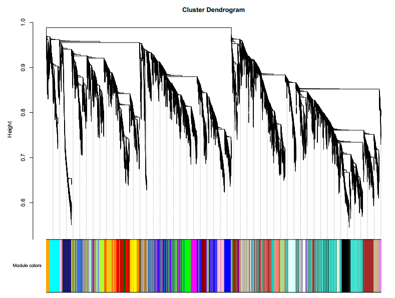
       横坐标：基因共表达模块分析的结果展示，不同的颜色代表不同的基因模块，灰色属于未知模块的基因

       纵坐标：基因间的不相似性系数，进化树的每一个树枝代表一个基因

4.2 NetworkHeatmap.pdf :共表达模块基因相关系数热图

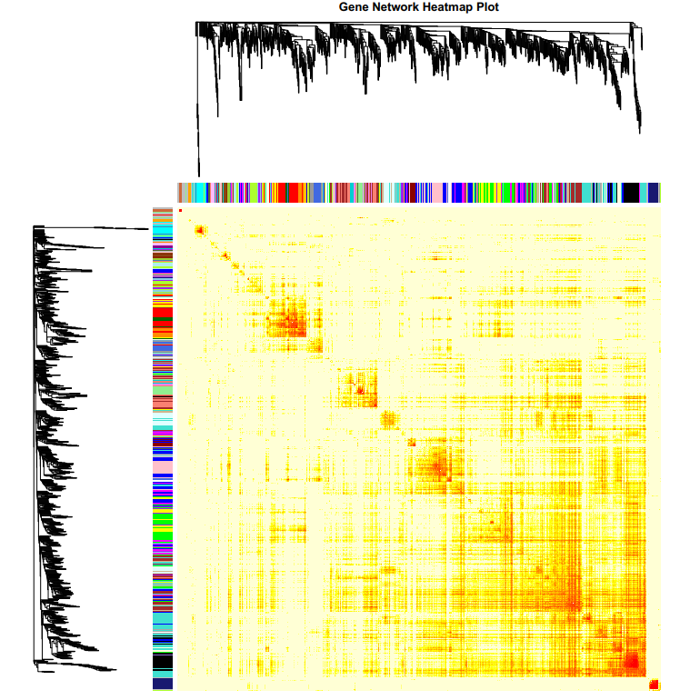
       图上和图左是基因系统发育树，每一个树枝代表一个基因，不同颜色亮带表示不同的module，每一个亮点表示每个基因与其他基因的相关性强弱，每个点的颜色越深（白→黄→红）代表行和列对应的两个基因间的连通性越强。P值采用student's t test计算所得，P值越小代表基因与模块相关性的显著性越强。

4.3 EigengeneDendrogramHeatmap.pdf :共表达模块的聚类图和热图

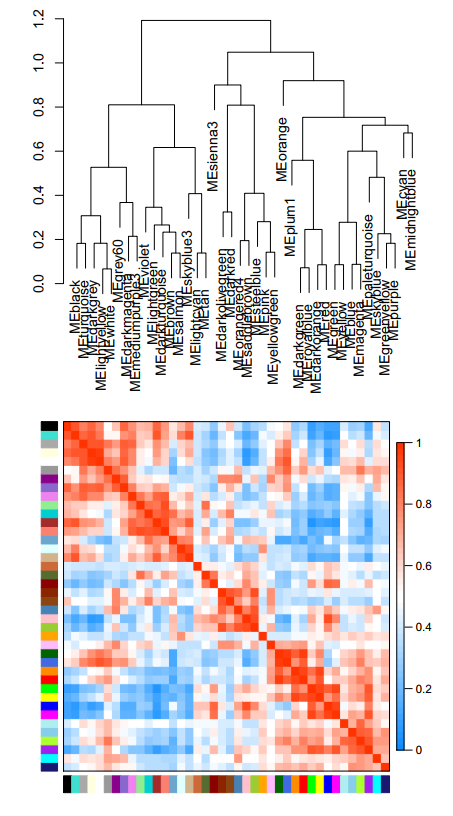
       聚类图：对每个基因模块的特征向量基因进行聚类,

       热图：我们将所有模块两两间的相关性进行分析，并绘制热图，颜色越红，相关性越高

4.4 ModuleSampleRelation.pdf : 性状相关特征模块分析（此分析需结合生理数据，如没有生理数据则没有此结果）

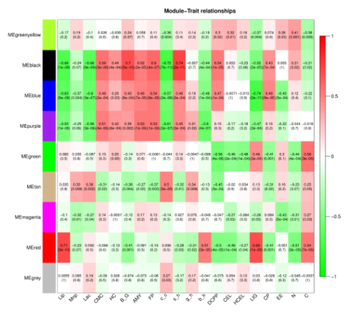
       每一列代表一个性状，每一行代表一个基因模块。每个格子里的数字代表模块与性状的相关性，该数值越接近1，表示模块与性状正相关性越强；越接近-1，表示模块与性状负相关性越强。括号里的数字代表显著性P value，该数值越小，表示显著性越强。P值采用student's t test计算所得，P值越小代表性状与模块相关性的显著性越强。