BEVFormer详解

BEVFormer 是什么

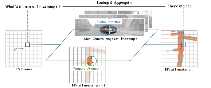
BEVFormer 是将Transformer架构的自注意机制与BEV视图中3D检测结合起来的一种纯视觉目标检测方案。

将Transformer架构的自注意力机制应用到目标检测方案有 DETR，deformable DETR，其中deformable DETR 首次将可变形稀疏局部自注意力代替Transform原版的全局自注意机制，使得训练推理计算更加高效。

基于BEV视图中3D检测方案起初均是为点云目标检测服务，流行的方法有PointNet++，PointPillar，centerPoint，大致的思路就是将3D点云拍扁的2D的BEV栅格上，然后类似图像的特征上进行分类和回归。

对于纯视觉的BEV检测方案，其中的重中之重就是如何将2D的图像特征映射到3D空间的BEV栅格，既然是映射关系，那就有前行投影和反向查询两种机制。前向投影是基于深度估计的方法，参考基于深度估计的BEV视图转换方法，典型代表为LSS。反向查询方法思路为先将BEV栅格在Z方向上进行lift提升，然后再映射到图像特征图上进行特征查询。BEVFormer 就是基于这种机制进行2D图像特征到3D空间的BEV栅格映射。

至于为什么要用BEV，什么是自注意力，什么是deformable attention，为什么要用纯视觉方案等等问题，这里不做详细解释，但是在看BEVformer之前，这些问题都是必现先搞明白的，特别是multiscale deformable attention ，因为整个BEVFormer最重要的encoder部分说白了就是在不停地做 deformable attention。

BEVFormer 流程

BEVFormer 的 Pipeline 分成几个部分：

1、Backbone: 主干网络提取图像多尺度特征。Backbone + FPN Neck 提取多个视角相机的多尺度特征。常用的有resnet50, resNet101-DCN等。
2、encoder: 完成2D图像多尺度特征映射到3D空间的BEV栅格。（包括 Temporal Self-Attention 模块和 Spatial Cross-Attention 模块。
3、Decoder: 在BEV栅格上完成 3D 目标检测的分类和定位任务， 类似Deformable DETR 的 Decoder
4、正负样本定义： 采用 Transformer 中常用的匈牙利匹配算法，Focal Loss + L1 Loss 的总损失和最小
5、损失函数： Focal Loss 分类损失 + L1 Loss 回归损失

BEVFormer 输入

输入的数据是一个 6 维的张量：（bs，queue，cam，C，H，W）；
bs: batchsize
queue：连续帧的个数；相当加入时序信息，起到多帧特征融合效果，对遮挡起到很好效果。所以加入网络的数据除当前帧之外，还有之前几帧的数据。
cam: 相机的个数，即每一帧包含图像的数量。例如nuScenes数据集而言，由于一辆车带有六个环视相机传感器，可以实现 360° 全场景的覆盖。cam = 6
C，H，W：图像通道数，图像高度，图像宽度

backbone 特征提取

提取某一帧对应的所有环视图像的多尺度特征。
对应代码如下，取出对应历史帧图像，将 bs * cam 作为新的bs送到backbone网络提取多尺度特征，返回后，再把 bs * cam 的维度再拆成 bs，cam。即可得到某一queue的特征。

# 输入图片信息 tensor: (bs, queue, cam, c, h, w)
# 通过 for loop 方式一次获取单帧对应的六张环视图像
# 送入到 Backbone + Neck 网络提取多尺度的图像特征

for idx in range(tensor.size(1) - 1):  # 利用除当前帧之外的所有帧迭代计算 `prev_bev` 特征
    single_frame = tensor[:, idx, :]   # (bs, cam, c, h, w)
    # 将 bs * cam 看作是 batch size，将原张量 reshape 成 4 维的张量
    # 待 Backbone + Neck 网络提取多尺度特征后，再把 bs * cam 的维度再拆成 bs，cam

    single_frame = single_frame.reshape(bs * cam, c, h, w)
    feats = Backbone(FPN(single_frame)) 

    """ feats 是一个多尺度的特征列表 """
    [0]: (bs, cam, 256, h / 8, w / 8)
    [1]: (bs, cam, 256, h / 16, w / 16)
    [2]: (bs, cam, 256, h / 32, w / 32)
    [3]: (bs, cam, 256, h / 64, w / 64)

encoder 核心

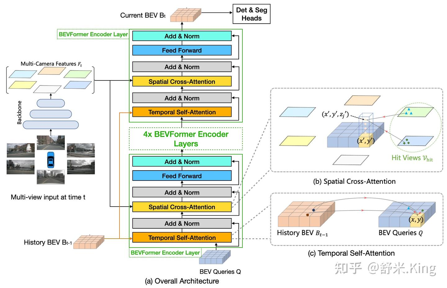
包含两个子模块 Temporal Self-Attention模块 以及 Spatial Cross-Attention模块；

Temporal Self-Attention 模块

主要做时序特征融合。

BEV Query 是什么？

可以理解 BEV Query 就是当前BEV特征。首先它是预定义的一组栅格（grid-shaped）可学习参数， $Q\in R^{H\times W\times C}$，它是对BEV感知空间的特征描述，当它完成学习以后，就变成了BEV 特征。

在Temporal Self-Attention模块，我们把历史BEV特征作为输入，与当前时刻的 BEV Query 进行融合，输出当前的 deformable attention 的Query特征。

对于一个deformable attention 模块，它处理数据的pipline 大致如下：

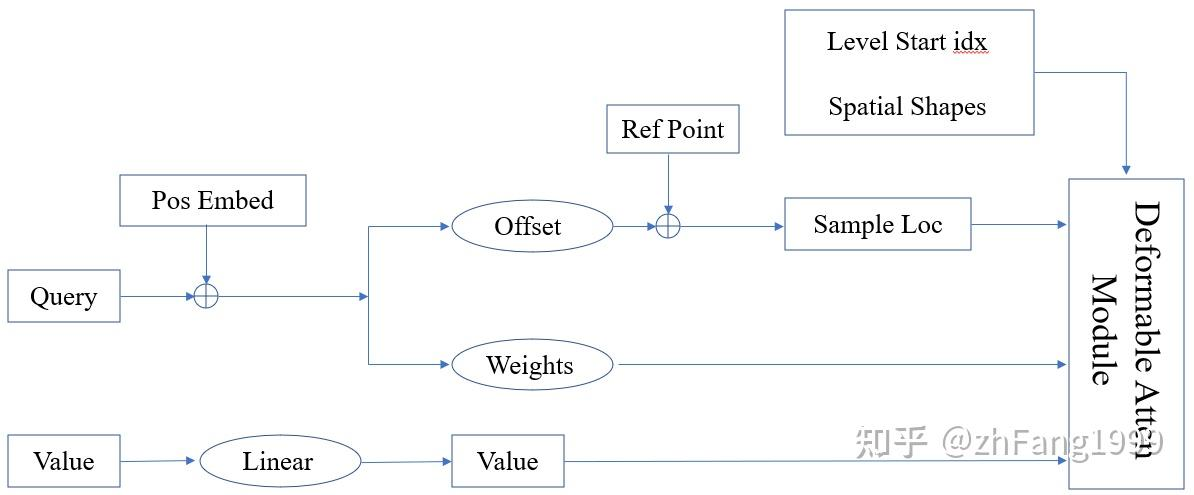
Deformable Attention Module CUDA 模块的输入分别是采样位置（Sample Location）、注意力权重（Attention Weights）、映射后的 Value 特征、多尺度特征每层特征起始索引位置、多尺度特征图的空间大小（便于将采样位置由归一化的值变成绝对位置）；

对于 Temporal Self-Attention 模块而言，需要 bev_query、bev_pos、prev_bev、ref_point、value等参数（需要用到的参数参考 Deformable Attention Pipeline 图解）

代码实现：

bev_query：

一个完全 learnable parameter，通过 nn.Embedding() 函数得到，形状 shape = (200 * 200，256)；200，200 分别代表 BEV 特征平面的长和宽。

bev_pose：

一个完全 learnable parameter。先分别产生行、列编码，再通过 cat 形成二维位置编码，相比直接生成二维位置编码节省了大量参数。

""" bev_pose 的生成过程 """
# w, h 分别代表 bev 特征的空间尺寸 200 * 200
x = torch.arange(w, device=mask.device)
y = torch.arange(h, device=mask.device)

# self.col_embed 和 self.row_embed 分别是两个 Linear 层，将(200, )的坐标向高维空间做映射
x_embed = self.col_embed(x)  # (200, 128)
y_embed = self.row_embed(y)  # (200, 128)

# pos shape: (bs, 256, 200, 200)
pos = torch.cat((x_embed.unsqueeze(0).repeat(h, 1, 1), y_embed.unsqueeze(1).repeat(1, w, 1)), dim=-1).permute(2, 0, 1).unsqueeze(0).repeat(mask.shape[0], 1, 1, 1)

prev_bev

历史时刻BEV特征

ref_point

ref_point 是参考点，也就是说当前BEV特征需要参考前一时刻的 BEV 特征的位置。
如果没有输入 prev_bev（第一帧没有前一时刻的 BEV 特征）的情况，其 ref_point = ref_2d；
对于存在输入 prev_bev 的情况，其 ref_point = ref_2d + shift；

ref_2d 是在相对BEV网格下的归一化坐标位置，即对于每一个BEV网格整型索引（i，j）都对应一个归一化的二维坐标位置。

shift 是历史帧BEV 相对当前帧 BEV的偏移

由于车身不断运动，而BEV是相对自车建立起来的坐标系，所以前后 BEV 在空间上的特征是不对齐的。为了实现两个时刻特征的空间对齐，需要用到 can_bus 数据中有关车自身旋转角度和偏移的信息。根据车辆的CAN_bus数据，计算从上一帧到当前帧的平移距离(translation_length)、平移方向(translation_angle)和旋转角度(bev_angle)。

对于相对车也在运动的物体的特征，这部分对齐需要自注意力模块去学习和修正。

"""shift 参数的生成""" 
# obtain rotation angle and shift with ego motion
 delta_x = kwargs['img_metas'][0]['can_bus'][0]
 delta_y = kwargs['img_metas'][0]['can_bus'][1]
 ego_angle = kwargs['img_metas'][0]['can_bus'][-2] / np.pi * 180
 rotation_angle = kwargs['img_metas'][0]['can_bus'][-1]
 grid_length_y = grid_length[0]
 grid_length_x = grid_length[1]
 translation_length = np.sqrt(delta_x ** 2 + delta_y ** 2)
 translation_angle = np.arctan2(delta_y, delta_x) / np.pi * 180
 if translation_angle < 0:
     translation_angle += 360
 bev_angle = ego_angle - translation_angle
 shift_y = translation_length * \
     np.cos(bev_angle / 180 * np.pi) / grid_length_y / bev_h
 shift_x = translation_length * \
     np.sin(bev_angle / 180 * np.pi) / grid_length_x / bev_w
 shift_y = shift_y * self.use_shift
 shift_x = shift_x * self.use_shift
 shift = bev_queries.new_tensor([shift_x, shift_y])  # shape (2,) 

# 通过`旋转`和`平移`变换实现 BEV 特征的对齐，对于平移部分是通过对参考点加上偏移量`shift`体现的
if prev_bev is not None:
    if prev_bev.shape[1] == bev_h * bev_w:
        prev_bev = prev_bev.permute(1, 0, 2)
    if self.rotate_prev_bev:
        num_prev_bev = prev_bev.size(1)
        prev_bev = prev_bev.reshape(bev_h, bev_w, -1).permute(2, 0, 1)  # sequence -> grid
        prev_bev = rotate(prev_bev, rotation_angle, center=self.rotate_center)
        prev_bev = prev_bev.permute(1, 2, 0).reshape(bev_h * bev_w, num_prev_bev, -1)

"""ref_2d 参数的生成，常规的 2D 网格生成的规则坐标点"""
ref_y, ref_x = torch.meshgrid(torch.linspace(0.5, H - 0.5, H, dtype=dtype, device=device),
                              torch.linspace(0.5, W - 0.5, W, dtype=dtype, device=device))
ref_y = ref_y.reshape(-1)[None] / H
ref_x = ref_x.reshape(-1)[None] / W
ref_2d = torch.stack((ref_x, ref_y), -1)
ref_2d = ref_2d.repeat(bs, 1, 1).unsqueeze(2)

value

value 就是对应着bev_query去查询的特征。

当存在prev_bev时， value = [prev_bev，bev_query]， ref_point = [ref_2d + shift，ref_2d], 将当前bev_query 与历史BEV特征融合。

当不存在prev_bev时，value = [bev_query，bev_query]，ref_point = [ref_2d，ref_2d]。

bev_query = [value[0]，bev_query]

所以整个attention 计算的是prev_bev以及bev_query自身的相似性，最后得到的两组bev_query结果做一下平均，得到当前attetion 输出。

进入到内部 Deformable Attention Module CUDA 模块 时的内部参数 Offset、Weights、 Sample Location 都是由前面的参数学习或计算得到。

最后 level = 1 。在deformable attention 中提到 level 为多尺度特征的层数，这里BEV特征只有一层，且代表真实3D空间信息，不需要多尺度。所以level = 1。

所以在进入 Deformable Attention Module CUDA 模块前的运算如下：

""" bev_query 按照通道维度进行 concat """  
query = torch.cat([value[0:1], query], -1)  # (bs, 40000, 512) 初始query 256 维， 月value[0] cat 后变成 512 维
""" value 经过 Linear 做映射 """
value = self.value_proj(value)
""" offsets 以及 attention weights 的生成过程 """
# sampling_offsets: shape = (bs, num_query, 8, 1, 4, 2)  # num_query=200*200， 8个head， layer = 1， 每个点采样个数为 4 
# 对 query 进行维度映射得到采样点的偏移量
sampling_offsets = self.sampling_offsets(query).view(bs, num_query, self.num_heads, self.num_levels, self.num_points, 2)
# 对 query 进行维度映射得到注意力权重
attention_weights = self.attention_weights(query).view(bs, num_query, self.num_heads, self.num_levels * self.num_points)  
attention_weights = attention_weights.softmax(-1)
# attention_weights: shape = (bs, num_query, 8, 1, 4)
attention_weights = attention_weights.view(bs, num_query, self.num_heads, self.num_levels, self.num_points) 
""" sample location 的生成过程 
通过代码可以观察到两点：
1. 通过 query 学到的 sampling_offsets 偏移量是一个绝对量，不是相对量，所以需要做 normalize；
2. 最终生成的 sampling_locations 是一个相对量；
"""
offset_normalizer = torch.stack([spatial_shapes[..., 1], spatial_shapes[..., 0]], -1)
sampling_locations = reference_points[:, :, None, :, None, :] \
                + sampling_offsets / offset_normalizer[None, None, None, :, None, :]

进入 Deformable Attention Module CUDA 模块运算，输出bev query

""" 各个参数的 shape 情况 
1. value: (2，40000，8，32） # 2: 代表前一时刻的 BEV 特征和后一时刻的 BEV 特征，两个特征在计算的过程中是互不干扰的，
                             # 40000: 代表 bev_query 200 * 200 空间大小的每个位置
                             # 8: 代表8个头，# 32: 每个头表示为 32 维的特征
2. spatial_shapes: (200, 200) # 方便将归一化的 sampling_locations 反归一化
3. level_start_index: 0 # BEV 特征只有一层
4. sampling_locations: (2, 40000, 8, 1, 4, 2)
5. attention_weights: (2, 40000, 8, 1, 4)

6. output: (2, 40000, 8, 32)
"""
output = MultiScaleDeformableAttnFunction.apply(value, 
                                                spatial_shapes, 
                                                level_start_index, 
                                                sampling_locations,
                                                attention_weights, 
                                                self.im2col_step)

""" 最后将前一时刻的 bev_query 与当前时刻的 bev_query 做平均
output = output.permute(1, 2, 0)
output = (output[..., :bs] + output[..., bs:])/self.num_bev_queue

output 就是当前时刻经过 Temporal Self-Attention 模块输出的bev_query，将作为Spatial Cross-Attention 模块的输入。

Spatial Cross-Attention 模块

Spatial Cross-Attention 将图像特征加进来，将2D的多尺度图像特征映射到BEV栅格上。

query 查询机制

Spatial Cross-Attention 采用的是反向查询机制获得图像特征。同时它查询的位置信息不是单纯通过内外参获得的固定位置，而是类似deformable attention 的方式通过学习offset获得参考点周围信息的查询位置。而参考点就是通过内外参建立起来的。

所以Spatial Cross-Attention 其实也是一个deformable attention 机制。它的输入输出与Temporal Self-Attention 相似。不同的是不需要 bev_pos 参数，因为它的bev_query 来自Temporal Self-Attention 的输出，已经添加了bev_pos 信息。只需要 bev_query、ref_point、value（就是 concat 到一起的多尺度图像特征）

bev_query

来自Temporal Self-Attention 的输出。

value

多尺度图像特征，这一部分在multiscale deformable attention 中介绍过， 就是将各个尺度的图像特征flatten()展平，然后concat 在一起作为value, 方便后面的查询。

图像特征加入相机编码 和 尺度层 编码 然后flatten() 、 concat(), 并记下每个特征层的起止位置，后面的查询需要。

""" 首先将多尺度的特征每一层都进行 flatten() """
for lvl, feat in enumerate(mlvl_feats):
    bs, num_cam, c, h, w = feat.shape
    spatial_shape = (h, w)
    feat = feat.flatten(3).permute(1, 0, 3, 2)  # (cam, bs, sum(h*w), 256)
    if self.use_cams_embeds:    #图像特征加入相机编码
        feat = feat + self.cams_embeds[:, None, None, :].to(feat.dtype)
        feat = feat + self.level_embeds[None, None, lvl:lvl + 1, :].to(feat.dtype) #图像特征加入特征层编码
        spatial_shapes.append(spatial_shape)
        feat_flatten.append(feat)

""" 对每个 camera 的所有层级特征进行汇聚 """
feat_flatten = torch.cat(feat_flatten, 2)  # (cam, bs, sum(h*w), 256)
spatial_shapes = torch.as_tensor(spatial_shapes, dtype=torch.long, device=bev_pos.device)

# 计算每层特征的起始索引位置
level_start_index = torch.cat((spatial_shapes.new_zeros((1,)), spatial_shapes.prod(1).cumsum(0)[:-1]))

# 维度变换
feat_flatten = feat_flatten.permute(0, 2, 1, 3)  # (num_cam, sum(H*W), bs, embed_dims)

ref_point

因为我们查询的是2D的图像特征，所以参考点当然是对应到图像上，所以实际的 参考点是 reference_points_cam。

但是3D的BEV空间如何对应到2D的图像上，就需要通过相机内外参进行建模。

1、首先建立3维坐标参考点 ： ref_3d坐标点

我们的bev_query 是2维的栅格，我们需要把它与真实自车坐标下的空间联系起来，并以此建立query对应的3维坐标参考点。
（1）、在BEV栅格Z轴方向上进行 lift 提升，选取4个坐标点，这样就是获得了BEV空间的高度信息，进而能映射到对应的高度特征。

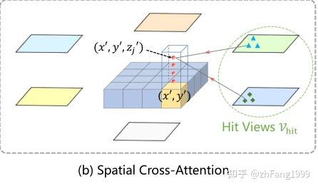
（2）、根据BEV空间的建模范围（实际检测的空间距离：前、后、左、右、上）将对应的实际空间坐标对应到 BEV 3维网格上得到ref_3d。

""" ref_3d 坐标生成 """
zs = torch.linspace(0.5, Z - 0.5, num_points_in_pillar, dtype=dtype, device=device).view(-1, 1, 1).expand(num_points_in_pillar, H, W) / Z
xs = torch.linspace(0.5, W - 0.5, W, dtype=dtype, device=device).view(1, 1, W).expand(num_points_in_pillar, H, W) / W
ys = torch.linspace(0.5, H - 0.5, H, dtype=dtype, device=device).view(1, H, 1).expand(num_points_in_pillar, H, W) / H
ref_3d = torch.stack((xs, ys, zs), -1)  # (4, 200, 200, 3)  (level, bev_h, bev_w, 3) 3代表 x,y,z 坐标值
ref_3d = ref_3d.permute(0, 3, 1, 2).flatten(2).permute(0, 2, 1)  # (4, 200 * 200, 3)
ref_3d = ref_3d[None].repeat(bs, 1, 1, 1)  # (1, 4, 200 * 200, 3)
# ref_3d:
#   zs: (0.5 ~ 8-0.5) / 8
#   xs: (0.5 ~ 50-0.5) / 50
#   ys: (0.5 ~ 50-0.5) / 50
# return ref_3d
# ----------------------get_reference_points end----------------------
# ref_2d = self.get_reference_points(
#     bev_h, bev_w, dim='2d', bs=bev_query.size(1), device=bev_query.device, dtype=bev_query.dtype)
# ---------------------get_reference_points start---------------------
ref_y, ref_x = torch.meshgrid(
 torch.linspace(
     0.5, bev_h - 0.5, bev_h, dtype=dtype, device=device),
 torch.linspace(
     0.5, bev_w - 0.5, bev_w, dtype=dtype, device=device)
)
ref_y = ref_y.reshape(-1)[None] / bev_h
ref_x = ref_x.reshape(-1)[None] / bev_w
ref_2d = torch.stack((ref_x, ref_y), -1)
ref_2d = ref_2d.repeat(bs, 1, 1).unsqueeze(2)  # ref_2d其实就是ref_3d torch.Size([1, 4(4个高度), 50*50, 3(x,y,z)]) 去掉高度的一部分，
# bs, bev_h * bev_w, None, xy # torch.Size([1, 50*50, 1, 2])
# return ref_2d
# ----------------------get_reference_points end----------------------
# reference_points_cam, bev_mask = self.point_sampling(ref_3d, self.pc_range, kwargs['img_metas'])

2、ref_3d坐标点投影到图像坐标上 ： ref_3d 映射到 reference_points_cam

由于一个3d 点可能会被多个相机看到，所以需要将每一个3d 点都往所有的图像上投影，得到图像特征参考点，最后再通过 mask 筛选出有效的投影，得到reference_points_rebatch 。

ref_3d 映射到 reference_points_cam 代码如下：

""" BEV 空间下的三维坐标点向图像空间转换的过程
代码中的`lidar2img`需要有两点需要注意
1. BEV 坐标系 这里指 lidar 坐标系
2. 这里提到的`lidar2img`是经过坐标变换的，一般分成三步
   第一步：lidar 坐标系 -> ego vehicle 坐标系
   第二步：ego vehicle 坐标系 -> camera 坐标系
   第三部：camera 坐标系 通过相机内参 得到像素坐标系
   以上这三步用到的所有平移和旋转矩阵都合并到了一起，形成了 `lidar2img` 旋转平移矩阵

同时需要注意：再与`lidar2img`矩阵乘完，还需要经过下面两步坐标系转换，才是得到了三维坐标点在二维图像平面上的点
"""
 # ------------------------point_sampling start------------------------
reference_points = ref_3d
# NOTE: close tf32 here.
allow_tf32 = torch.backends.cuda.matmul.allow_tf32
torch.backends.cuda.matmul.allow_tf32 = False
torch.backends.cudnn.allow_tf32 = False

lidar2img = []      
for img_meta in ohb_img_metas:
    lidar2img.append(img_meta['lidar2img'])  # lidar2img 激光雷达到图像坐标的转换，将激光雷达坐标系当作自车坐标系
lidar2img = np.asarray(lidar2img)
lidar2img = reference_points.new_tensor(lidar2img)  # torch.Size([1, 6, 4, 4]) 相机内外参合成一个矩阵4*4
reference_points = reference_points.clone()
# reference_points = ref_3d # normalize 0~1 # torch.Size([1, 4, 50*50, 3])
# pc_range = [-51.2, -51.2, -5.0, 51.2, 51.2, 3.0]  长102.4  宽102.4  高8
# 映射到自车坐标系下, 尺度被反归一化为真实尺度(米)   
reference_points[..., 0:1] = reference_points[..., 0:1] * \
    (pc_range[3] - pc_range[0]) + pc_range[0]  # x 0~1 缩放到 0~102.4
reference_points[..., 1:2] = reference_points[..., 1:2] * \
    (pc_range[4] - pc_range[1]) + pc_range[1]  # y 0~1 缩放到 0~102.4
reference_points[..., 2:3] = reference_points[..., 2:3] * \
    (pc_range[5] - pc_range[2]) + pc_range[2]  # z 0~1 缩放到 0~8

# 变成齐次坐标
reference_points = torch.cat((reference_points, torch.ones_like(reference_points[..., :1])), -1)
# bs, num_points_in_pillar, bev_h * bev_w, xyz1  齐次坐标通过升维将平移纳入矩阵乘法 [x,y,z]-->[x,y,z,1]齐次坐标形式，为了和lidar2img[1, 6, 4, 4]做乘法
reference_points = reference_points.permute(1, 0, 2, 3)
# num_points_in_pillar, bs, bev_h * bev_w, xyz1
D, B, num_query = reference_points.size()[:3]
num_cam = lidar2img.size(1)  # 6
reference_points = reference_points.view(D, B, 1, num_query, 4).repeat(1, 1, num_cam, 1, 1).unsqueeze(-1)
ref_3d = ref_3d[None].repeat(bs, 1, 1, 1)  # bs, num_points_in_pillar, bev_h * bev_w, xyz # torch.Size([1, 4, 50*50, 3])
 # bs, num_points_in_pillar, bev_h * bev_w, xyz # torch.Size([1, 4, 50*50, 3])
lidar2img = lidar2img.view(1, B, num_cam, 1, 4, 4).repeat(D, 1, 1, num_query, 1, 1)
# num_points_in_pillar, bs, num_cam, bev_h * bev_w, 4, 4   

reference_points_cam = torch.matmul(lidar2img.to(torch.float32), reference_points.to(torch.float32)).squeeze(-1)  # 每个 3D 点投影到 6 个相机上的齐次坐标 (u, v, s, 1)
# num_points_in_pillar, bs, num_cam, bev_h * bev_w, uvs1  s代表比例（x,y,s == kx,ky,ks  s==1，x/s, y/s）

从3D投影到2D判断是否有效有两个条件：

1、投影射线与图像相交相机正前方，判断条件为 reference_points_cam[…, 2:3] > 0
2、投影射线与相机平面相交在像素范围内 , 归一化后的判断条件为：
(reference_points_cam[…, 1:2] > 0.0)
& (reference_points_cam[…, 1:2] < 1.0)
& (reference_points_cam[…, 0:1] < 1.0)
& (reference_points_cam[…, 0:1] > 0.0))

eps = 1e-5
# (level, bs, cam, num_query, 1)
bev_mask = (reference_points_cam[..., 2:3] > eps)  # 只保留位于相机前方的点
# 齐次坐标下除以比例系数得到图像平面的坐标真值 : 将投影结果从 (u, v, s) 转换为实际的 2D 像素坐标 (x, y)
reference_points_cam = reference_points_cam[..., 0:2] / torch.maximum(
    reference_points_cam[..., 2:3], torch.ones_like(reference_points_cam[..., 2:3]) * eps)
# num_points_in_pillar, bs, num_cam, bev_h * bev_w, uv

# 坐标归一化 都在0-1之间
reference_points_cam[..., 0] /= ohb_img_metas[0]['img_shape'][0][1]
reference_points_cam[..., 1] /= ohb_img_metas[0]['img_shape'][0][0]

# 去掉图像以外的点  先保证uv坐标都在0-1之间【在相机的视场内】  num_points_in_pillar, bs, num_cam, bev_h * bev_w, uv
bev_mask = (bev_mask & (reference_points_cam[..., 1:2] > 0.0)
            & (reference_points_cam[..., 1:2] < 1.0)
            & (reference_points_cam[..., 0:1] < 1.0)
            & (reference_points_cam[..., 0:1] > 0.0))

前面获得了 bev_query , reference_points_cam, 实际应用上我们是通过 bev_mask 选取有用的参考点进行计算，提高计算效率和训练的收敛速度。所以将 bev_query 整合成 queries_rebatch， reference_points_cam 整合成 reference_points_rebatch 进行计算。

bev_query 到 queries_rebatch
reference_points_cam 到 reference_points_rebatch

bev_mask : shape(cam=6, num_query=200200, level=4)
query: shape(bs=2, num_query=200200，256)
reference_points_cam: shape(cam=6, num_query=200*200, level=4 , xy = 2)

bev_mask 存储了 BEV 立体网格到每个相机的有效映射。例如一个BEV立体（x * y，z）, 在第0、1个cam 上有映射，在第2、3个cam 上没有映射。所以对于任意一个BEV栅格下（x, y）映射到某个相机上，然后在Z方向上求和，为0说明 BEV栅格（x,y）在此相机没有有效映射。也就是说当前（x,y）处对应的bev_query 在此相机无效。依据这种方法，找到每一个相机上有效的bev_query 和有效的reference_points_cam。
对应代码为： index_query_per_img = mask_per_img[0].sum(-1).nonzero().squeeze(-1)

例如每个cam有效bev_query 索引如下：
cam0: 0,1,2,3… 100
cam1: 50,51,52… 100, 101, 150
cam2:100,101,…200
…
也就是 BEV 栅格索引为50的能同时被cam0 和 cam1同时看到，索引为120的能同时被cam1 和 cam2同时看到， 以此类推

得到每个相机的有效索引后，构建所有相机的queries_rebatch和reference_points_rebatch。
对应代码为：queries_rebatch[j * self.num_cams + i, :len(index_query_per_img)] = query[j, index_query_per_img]

indexes = []
# 根据每张图片对应的`bev_mask`结果，获取有效query的index
for i, mask_per_img in enumerate(bev_mask):
    index_query_per_img = mask_per_img[0].sum(-1).nonzero().squeeze(-1)  # 获得每个相机的有效query的index
    indexes.append(index_query_per_img) # 为每个相机存储有效的query index

queries_rebatch = query.new_zeros([bs * self.num_cams, max_len, self.embed_dims]) #构建 queries_rebatch， 假设每个相机对应的最大有效query个数为max_len
reference_points_rebatch = reference_points_cam.new_zeros([bs * self.num_cams, max_len, D, 2]) 

for i, reference_points_per_img in enumerate(reference_points_cam):
    for j in range(bs):
        index_query_per_img = indexes[i]

        # 重新整合 `bev_query` 特征，记作 `query_rebatch， 为每个相机赋予响应的有效query
        queries_rebatch[j * self.num_cams + i, :len(index_query_per_img)] = query[j, index_query_per_img]

        # 重新整合 `reference_point`采样位置，记作`reference_points_rebatch`
        reference_points_rebatch[j * self.num_cams + i, :len(index_query_per_img)] = reference_points_per_img[j, index_query_per_img]

产生进入Deformable Attention Module CUDA 模块前的内部参数

有queries_rebatch和reference_points_rebatch之后，就可以类似Temporal Self-Attention 一样去产生内部参数Offset、Weights、Sample Locations
下面用的 query 指代的是上面提到的 quries_rebatch， num_query = max_len。

""" 获取 sampling_offsets，依旧是对 query 做 Linear 做维度的映射，但是需要注意的是
这里的 query 指代的是上面提到的 `quries_rebatch` """
 # sample 8 points for single ref point in each level.

# sampling_offsets: shape = (bs, max_len, 8, 4, 8, 2)
sampling_offsets = self.sampling_offsets(query).view(bs, num_query, self.num_heads, self.num_levels, self.num_points, 2)
attention_weights = self.attention_weights(query).view(bs, num_query, self.num_heads, self.num_levels * self.num_points)
attention_weights = attention_weights.softmax(-1)
# attention_weights: shape = (bs, max_len, 8, 4, 8)
attention_weights = attention_weights.view(bs, num_query,
                                           self.num_heads,
                                           self.num_levels,
                                           self.num_points)
""" 生成 sampling location """
offset_normalizer = torch.stack([spatial_shapes[..., 1], spatial_shapes[..., 0]], -1)
reference_points = reference_points[:, :, None, None, None, :, :]
sampling_offsets = sampling_offsets / offset_normalizer[None, None, None, :, None, :]
sampling_locations = reference_points + sampling_offsets

Spatial Cross-Attention 模块输出bev_embedding特征

在 queries_rebatch 和 reference_points_rebatch 上进行查询的，最后仍需要将这些分配到每一个相机上的query整合到统一的BEV栅格上，并且求平均获得当前BEV栅格的query。

例如 BEV栅格索引=50 处的能同时被cam0 和 cam1同时看到， 那它的query来自cam0 和 cam1。

对应代码：
slots[j, index_query_per_img] += queries[j * self.num_cams + i, :len(index_query_per_img)]

"""
1. value: shape = (cam = 6, sum(h_i * w_i) = 30825, head = 8, dim = 32)
2. spatial_shapes = ([[116, 200], [58, 100], [29,  50], [15,  25]])
3. level_start_index= [0, 23200, 29000, 30450]
4. sampling_locations = (cam, max_len, 8, 4, 8, 2)
5. attention_weights = (cam, max_len, 8, 4, 8)
6. output = (cam, max_len, 8, 32)
"""
output = MultiScaleDeformableAttnFunction.apply(value, spatial_shapes, level_start_index, sampling_locations,
                attention_weights, self.im2col_step)
"""最后再将六个环视相机查询到的特征整合到一起，再求一个平均值 """
for i, index_query_per_img in enumerate(indexes):
    for j in range(bs):  # slots: (bs, 40000, 256)
        slots[j, index_query_per_img] += queries[j * self.num_cams + i, :len(index_query_per_img)]
count = bev_mask.sum(-1) > 0
count = count.permute(1, 2, 0).sum(-1)
count = torch.clamp(count, min=1.0)
slots = slots / count[..., None]  # maybe normalize.
slots = self.output_proj(slots)

至此Spatial Cross-Attention 模块结束

将 Temporal Self-Attetion 模块和 Spatial Cross-Attention 模块堆叠在一起，当前 Spatial Cross-Attention 的 bev_embedding输出作为下一个Temporal Self-Attetion的输入， 并重复六次，最终得到的 BEV Embedding 特征作为下游 3D 目标检测和道路分割任务的 BEV 空间特征。

Decoder

decoder 的输入来自encoder 六次堆叠后的 bev_embedding 输出。

decoder 模块其实也是一次Deformable attention，与 Temporal Self-Attetion 类似，都是在BEV 2D 栅格上进行查询和输出。思想来自Deformable DETR 。

学习预测框和分类

用 object_query_embed 来学习预测框和分类， 模型直接用 nn.Embedding() 生成一组（900，512）维的张量，将 512 维的张量分成两组，分别构成了query = (900，256)和query_pos = (900，256)。即最多预测900个目标。

输入需要 query, query_pos, referece_points

预测过程没有参考点referece_points，因为没有先验，只能靠网络自己学习。referece_points学习参考点的信息来自query_pos。

reference_points = self.reference_points(query_pos)  # (bs, 900, 3)  3 代表 (x, y, z) 坐标
reference_points = reference_points.sigmoid()  # absolute -> relative
init_reference_out = reference_points 

decoder 的 Deformable attention 核心代码如下：

""" 由 query 生成 sampling_offsets 和 attention_weights """
sampling_offsets = self.sampling_offsets(query).view(
            bs, num_query, self.num_heads, self.num_levels, self.num_points, 2)  # (bs, 900, 8, 1, 4, 2)
attention_weights = self.attention_weights(query).view(
            bs, num_query, self.num_heads, self.num_levels * self.num_points)  # (bs, 900, 8, 4)
attention_weights = attention_weights.softmax(-1)
attention_weights = attention_weights.view(bs, num_query,
                                                   self.num_heads,
                                                   self.num_levels,
                                                   self.num_points)  # (bs, 900, 8, 1, 4)

""" sampling_offsets 和 reference_points 得到 sampling_locations """
offset_normalizer = torch.stack(
                [spatial_shapes[..., 1], spatial_shapes[..., 0]], -1)
sampling_locations = reference_points[:, :, None, :, None, :] \
                + sampling_offsets \
                / offset_normalizer[None, None, None, :, None, :]

""" 多尺度可变形注意力模块 """
# value: shape = (bs, 40000, 8, 32)
# spatial_shapes = (200, 200)
# level_start_index = 0
# sampling_locations = (bs, 900, 8, 1, 4, 2)
# attention_weights = (bs, 900, 8, 1, 4)

# output = (bs, 900, 256)
output = MultiScaleDeformableAttnFunction.apply(value, spatial_shapes, level_start_index, sampling_locations,
                attention_weights, self.im2col_step)

查询特征输出 output = (bs, 900, 256)

经过全连接层（FFN网络）进行目标的分类和回归。

回归预测 10 个维度的含义为：[xc，yc，w，l，zc，h，rot.sin()，rot.cos()，vx，vy]；[预测框中心位置的x方向偏移，预测框中心位置的y方向偏移，预测框的宽，预测框的长，预测框中心位置的z方向偏移，预测框的高，旋转角的正弦值，旋转角的余弦值，x方向速度，y方向速度]；

decoder 级联

然后根据预测的偏移量，对参考点的位置进行更新，为级联的下一个 Decoder 提高精修过的参考点位置，核心代码如下：

if reg_branches is not None:  # update the reference point.
    tmp = reg_branches[lid](output)  # (bs, 900, 256) -> (bs, 900, 10) 回归分支的预测输出
    assert reference_points.shape[-1] == 3
    new_reference_points = torch.zeros_like(reference_points)

    # 预测出来的偏移量是绝对量
    new_reference_points[..., :2] = tmp[..., :2] + inverse_sigmoid(reference_points[..., :2])  # 框中心处的 x, y 坐标
    new_reference_points[..., 2:3] = tmp[..., 4:5] + inverse_sigmoid(reference_points[..., 2:3])  # 框中心处的 z 坐标

    # 参考点坐标是一个归一化的坐标
    new_reference_points = new_reference_points.sigmoid()
    reference_points = new_reference_points.detach()

""" 
最后将每层 Decoder 产生的特征 = (bs, 900, 256)，以及参考点坐标 = (bs, 900, 3) 保存下来。
"""
if self.return_intermediate:
    intermediate.append(output)
    intermediate_reference_points.append(reference_points)

将层级的 bev_embedding特征以及参考点通过 for loop 的形式，一次计算每个 Decoder 层的分类和回归结果

bev_embed, hs, init_reference, inter_references = outputs
hs = hs.permute(0, 2, 1, 3)  # (decoder_level, bs, 900, 256)
outputs_classes = []
outputs_coords = []
for lvl in range(hs.shape[0]):
    if lvl == 0:
        reference = init_reference
    else:
        reference = inter_references[lvl - 1]
    reference = inverse_sigmoid(reference)
    outputs_class = self.cls_branches[lvl](hs[lvl])  # (bs, 900, num_classes)
    tmp = self.reg_branches[lvl](hs[lvl])  # (bs, 900, 10)
    assert reference.shape[-1] == 3
    tmp[..., 0:2] += reference[..., 0:2]  # (x, y)
    tmp[..., 0:2] = tmp[..., 0:2].sigmoid()
    tmp[..., 4:5] += reference[..., 2:3]
    tmp[..., 4:5] = tmp[..., 4:5].sigmoid()
    tmp[..., 0:1] = (tmp[..., 0:1] * (self.pc_range[3] - self.pc_range[0]) + self.pc_range[0])
    tmp[..., 1:2] = (tmp[..., 1:2] * (self.pc_range[4] - self.pc_range[1]) + self.pc_range[1])
    tmp[..., 4:5] = (tmp[..., 4:5] * (self.pc_range[5] - self.pc_range[2]) + self.pc_range[2])

    outputs_coord = tmp
    outputs_classes.append(outputs_class)
    outputs_coords.append(outputs_coord) 

正负样本的定义

正负样本的定义用到的就是匈牙利匹配算法，分类损失和类似回归损失的总损失和最小；

损失函数

分类损失：交叉熵

cls_pred = cls_pred.sigmoid()  # calculate the neg_cost and pos_cost by focal loss.
neg_cost = -(1 - cls_pred + self.eps).log() * (1 - self.alpha) * cls_pred.pow(self.gamma)
pos_cost = -(cls_pred + self.eps).log() * self.alpha * (1 - cls_pred).pow(self.gamma)
cls_cost = pos_cost[:, gt_labels] - neg_cost[:, gt_labels]
cls_cost = cls_cost * self.weight

回归损失：L1 Loss

self.reg_cost(bbox_pred[:, :8], normalized_gt_bboxes[:, :8])

参考链接：
万字长文理解纯视觉感知算法 —— BEVFormer
一文读懂BEVFormer论文
BEVFormer解读（提问版）