金融理论、投资组合与量化选股_18资产收益率和风险

1. 书籍和文中所提到的数据会在文末提供百度云下载，所有数据都不会有加密，可以放心下载使用
2. 文中计算的结果与书中不同是由于数据使用的时间段不同

目录

1. 单期与多期简单收益率

 2. 年化收益率

3. 连续复利收益率

4. 多期连续复利收益率

5. 单期与多期连续复利收益率的关系

 6. 绘制收益图

 7. 资产风险的测度——方差

8. 资产风险的测度——下行风险

 9. 资产风险的测度——风险价值

 10. 资产风险的测度——期望亏空

 11. 资产风险的测度——最大回撤

---

 

1. 单期与多期简单收益率

在计算单个资产的收益率或者比较不同资产的收益率时，我们需要先确定资产的持有期间。单期指收益率计算的时间间隔是一期，这里的一期可以以天为单位，也可以以月、季度或者年为单位。多期是指时间跨度为2期或2期以上。

计算万科1期和2期收益率

import pandas as pd
import numpy as np
df = pd.read_csv('./000002.csv',encoding='utf-8')
df.head()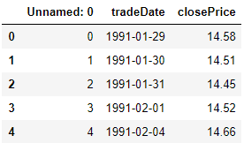

df['tradeDate'] = pd.to_datetime(df['tradeDate'])
df.sort_values(by='tradeDate',ascending=True,inplace=True)
df00 = df[df['tradeDate']>='2014-01-01']
df00 = df00.iloc[:311,:]
df00.head()

 

df00.set_index('tradeDate',inplace=True)
close = df00.closePrice
close.index.name='Date'
close.head()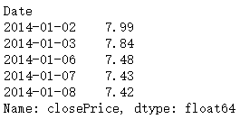

 

# 将收盘价滞后一期
lagclose = close.shift(1)
lagclose.head()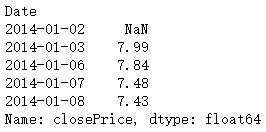

 

# 合并close , lagclose 这两个收盘价数据
Calclose = pd.DataFrame({'close':close,'lagclose':lagclose})
Calclose.head()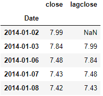

 

# 计算单期简单收益率
simpleret = (close-lagclose)/lagclose
simpleret.name = 'simpleret'
simpleret.head()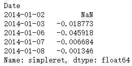

calret = pd.merge(Calclose,pd.DataFrame(simpleret),left_index=True,right_index=True)
calret.head()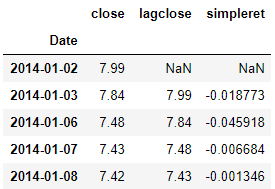

 

# 计算2期简单收益率
simpleret2 = (close-close.shift(2))/close.shift(2)
simpleret2.name = 'simpleret2'
calret['simpleret2'] = simpleret2
calret.head()

 

# 查看1月9日的数据
calret.iloc[5,:]

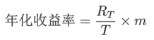
 2. 年化收益率

年化收益率的计算与复利相关，假设投资人持有资产时间为T期，获得的（或将要获得的）收益率为RT, 一年一共有m个单期（比如以月为单期，一年有12个月），则该资产的年化收益率为：

或

 

# 假设一年有245个交易日
annualize = (1+simpleret).cumprod()[-1]**(245/311)-1
annualize
# out: 0.5660614874349641

3. 连续复利收益率

 

# 计算单期连续复利收益率
comporet = np.log(close/lagclose)
comporet.name = 'comporet'
comporet.head()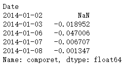

comporet[5]
# out: 0.005376357036380496

4. 多期连续复利收益率

# 多期连续复利收益率
comporet2 = np.log(close/close.shift(2))
comporet2.name='comporet2'
comporet2.head()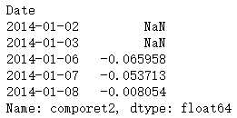

comporet2[5]
# out: 0.004029555486001642

5. 单期与多期连续复利收益率的关系

# 单期加总即得多期
comporet = comporet.dropna()
sumcomporet = comporet+comporet.shift(1)
sumcomporet.head()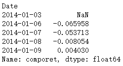

 6. 绘制收益图

simpleret.plot()

((1+simpleret).cumprod()-1).plot()

 7. 资产风险的测度——方差

# 数据日期为2014年1月1日到2014年12月21日
# 600343  航天动力
# 600346  大橡塑
df_600343 = pd.read_csv('./600343.csv',encoding='utf-8')
df_600346 = pd.read_csv('./600346.csv',encoding='utf-8')

df_600343['tradeDate'] = pd.to_datetime(df_600343['tradeDate'])
df_600343.sort_values(by='tradeDate',ascending=True,inplace=True)
df_600343_00 = df_600343[(df_600343['tradeDate']>='2014-01-01') & (df_600343['tradeDate']<='2014-12-31')]
df_600343_00.set_index('tradeDate',inplace=True)

df_600346['tradeDate'] = pd.to_datetime(df_600346['tradeDate'])
df_600346.sort_values(by='tradeDate',ascending=True,inplace=True)
df_600346_00 = df_600346[(df_600346['tradeDate']>='2014-01-01') & (df_600346['tradeDate']<='2014-12-31')]
df_600346_00.set_index('tradeDate',inplace=True)

returnS = (df_600343_00['closePrice']-df_600343_00['closePrice'].shift(1))/df_600343_00['closePrice'].shift(1)
returnD = (df_600346_00['closePrice']-df_600346_00['closePrice'].shift(1))/df_600346_00['closePrice'].shift(1)

returnS.std()
# out: 0.04275196558069479

returnD.std()
# out: 0.02092177691291706

8. 资产风险的测度——下行风险

# 比较两只股票的下行风险
def cal_half_dev(returns):
    mu = returns.mean()
    temp = returns[returns<mu]
    half_deviation=(sum((mu-temp)**2)/len(returns))**0.5
    return (half_deviation)

cal_half_dev(returnS)
# out: 0.036604972076999705

cal_half_dev(returnD)
# out: 0.014074947884289079

 9. 资产风险的测度——风险价值

# 历史模拟法
returnS.quantile(0.05)
# out: -0.043239530438867156

returnD.quantile(0.05)
# out: -0.03457604701374094

# 协方差矩阵法
from scipy.stats import norm
norm.ppf(0.05,returnS.mean(),returnS.std())
# out: -0.06821340640140308

norm.ppf(0.05,returnD.mean(),returnD.std())
# out: -0.0337355404401935

 10. 资产风险的测度——期望亏空

returnS[returnS<=returnS.quantile(0.05)].mean()
# out: -0.0337355404401935

returnD[returnD<=returnD.quantile(0.05)].mean()
# out: -0.04528445493770186

 11. 资产风险的测度——最大回撤

# 最大回撤
valueS = (1+returnS).cumprod()
valueS_D = valueS.cummax()-valueS
valueS_d = valueS_D/(valueS_D + valueS)
MMD_S = valueS_D.max()
# 最大回撤
MMD_S
# out: 0.7353951890034371
# 最大回撤率
mmd_S = valueS_d.max()
mmd_S
# out: 0.5676392572944298

PS:

书籍
链接：https://pan.baidu.com/s/1xJD85-LuaA9z-Jy_LU5nOw 
提取码：ihsg

链接：https://pan.baidu.com/s/1tF2RVDrHWNeniCLoploUTg 
提取码：1xmk