


针对(一)已经完成预处理后的数据,这里我采用了两套数据进行分析,由于涉及毕业设计内容,采用G1和G2代替预处理后的两套数据。下面展开对数据的注释、简单的浸润差异分析与Hallmarker功能差异分析。
第一步:数据读入
对(一)保存的数据进行读入,这里共两套数据
G1 <- readRDS(file = './G1_obj.RDS')
G2 <- readRDS(file = './G2_obj.RDS')
第二步:添加额外信息(meta信息)
需要对单细胞的meta信息进行添加的才进行这一步骤。这里对G1进行添加,如G2需要,步骤同下
Meta<- read.csv("./G1_Meta.csv")
Meta$Dataset <- "G1"
colnames(Meta)[1] <- "orig.ident"
row_name <- rownames(G1@meta.data)
G1@meta.data$id <- 1:nrow(G1@meta.data)
G1@meta.data <- merge(G1@meta.data, Meta, by = "orig.ident")
G1@meta.data <- G1@meta.data[order(G1@meta.data$id ),]
rownames(G1@meta.data) <- row_name
head(Meta,1)
注:这里使用merge会打乱数据框原有的顺序,因此采用提前添加id,之后进行排序完成顺序的校正,从而补上merge后缺失的行名
第三步:合并数据,并进行细胞自动注释与手动注释
合并数据并自动注释
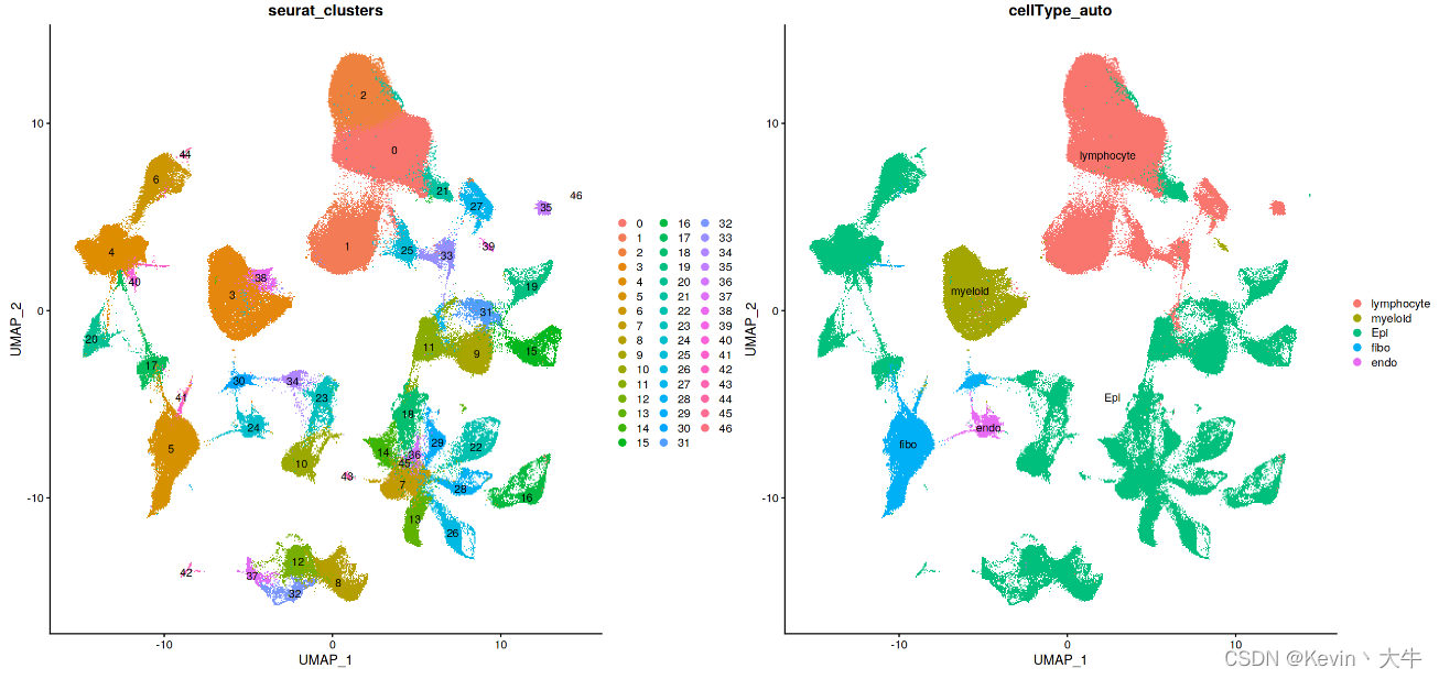
#合并数据,并进行预处理
BRCA_SingleCell.T <- merge(G1, G2)
rm(G1)
rm(G2)
BRCA_SingleCell.T <- NormalizeData(BRCA_SingleCell.T, normalization.method = "LogNormalize")
BRCA_SingleCell.T <- FindVariableFeatures(BRCA_SingleCell.T, selection.method = "vst", nfeatures = 3000)
BRCA_SingleCell.T <- ScaleData(BRCA_SingleCell.T, vars.to.regress = c('nCount_RNA'))
BRCA_SingleCell.T <- RunPCA(BRCA_SingleCell.T)
BRCA_SingleCell.T <- RunHarmony(object = BRCA_SingleCell.T,group.by.vars = c('Dataset'))
BRCA_SingleCell.T <- RunUMAP(BRCA_SingleCell.T,reduction = "harmony",dims = 1:30,seed.use = 12345)
BRCA_SingleCell.T <- FindNeighbors(BRCA_SingleCell.T,reduction = 'harmony', dims = 1:30, verbose = FALSE)
BRCA_SingleCell.T <- FindClusters(BRCA_SingleCell.T,resolution = 0.5, verbose = FALSE,random.seed=20220727)
#对合并数据重新进行细胞自动注释
cellAnnotation <- function(obj,markerList,assay='SCT',slot='data'){
    markergene <- unique(do.call(c,markerList))
    Idents(obj) <- 'seurat_clusters'
    cluster.averages <- AverageExpression(obj,assays=assay, slot = slot,features=markergene, return.seurat = TRUE)
    if(assay=='SCT'){
        scale.data <- cluster.averages@assays$SCT@data
    }else{
        scale.data <- cluster.averages@assays$RNA@data
    }
    print(scale.data)
    cell_score <- sapply(names(markergeneList),function(x){
        tmp <- scale.data[rownames(scale.data)%in%markergeneList[[x]],]
        if(is.matrix(tmp)){
            if(nrow(tmp)>=2){
                res <- apply(tmp,2,max)
                return(res)
            }else{
                return(rep(-2,ncol(tmp)))
            }
        }else{
            return(tmp)
        }
    })
    print(cell_score)
    celltypeMap <- apply(cell_score,1,function(x){
        colnames(cell_score)[which(x==max(x))]
    },simplify = T)
    obj@meta.data$cellType_auto <- plyr::mapvalues(x = obj@active.ident, from = names(celltypeMap), to = celltypeMap)
    return(obj)
}
lymphocyte <- c('CD3D','CD3E','CD79A','MS4A1','MZB1')
myeloid <- c('CD68','CD14','TPSAB1' , 'TPSB2','CD1E','CD1C','LAMP3', 'IDO1')
EOC <- c('EPCAM','KRT19','CD24')
fibo_gene <- c('DCN','FAP','COL1A2')
endo_gene <- c('PECAM1','VWF')
markergeneList <- list(lymphocyte=lymphocyte,myeloid=myeloid,Epi=EOC,fibo=fibo_gene,endo=endo_gene)
BRCA_SingleCell.T <- cellAnnotation(obj=BRCA_SingleCell.T,assay = 'RNA',markerList=markergeneList)
合并之后可视化合并后的数据
展示细胞簇的基因表达情况
genes_to_check = c('PTPRC', 'CD3D', 'CD3E', 'CD4','CD8A','TNFRSF18','SLC4A10','IL7R',
                   'CD19', 'CD79A', 'MS4A1' ,
                   'IGHG1', 'MZB1', 'SDC1',
                   'CD68', 'CD163', 'CD14', 'JCHAIN',
                   'TPSAB1' , 'TPSB2',
                   'RCVRN','FPR1' , 'ITGAM' ,
                   'C1QA',  'C1QB',
                   'S100A9', 'S100A8','CD86', 'MMP19',
                   'LAMP3', 'IDO1','IDO2',
                   'CD1E','CD1C',
                   'KRT86','GNLY',
                   'FGF7','MME','ACTA2','GFPT2','CNN1','CNN2',
                   'DCN', 'LUM',  'GSN' ,
                   'FAP','FN1','THY1','COL1A1','COL3A1',
                   'PECAM1', 'VWF',
                   'EPCAM' , 'KRT19', 'PROM1', 'CD24','MKI67',
                   'ALDH1A1', 'ALDH1A3','ITGA4','ITGA6')
DotPlot(BRCA_SingleCell.T,group.by = 'seurat_clusters', features = unique(genes_to_check),cluster.idents = T) + coord_flip()
结果如下:
根据基因表达图,手动注释细胞类型
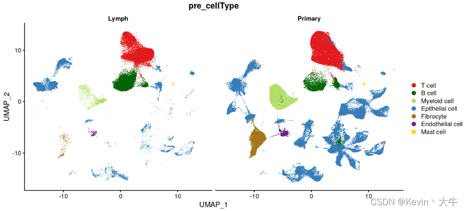
B_P_cell=c(1,25,36)
Mast_cell=c(39)
T_cell=c(0,2)
Epithelial=c(14,10,11,23,31,46,21,28,30,35,32,7,18,16,26,17,19,43,45,22,12,33,42,20,44,8,29,6,9,4,15,40,13,37)
Endothelial =c(24)
Myeloid=c(3)
Fibro_cell=c(5,47)
MIX=c(38,27,34,41)
table(c(B_P_cell,Mast_cell,T_cell,Epithelial,Endothelial,Myeloid,Fibro_cell,MIX))
print(setdiff(0:47,c(B_P_cell,Mast_cell,T_cell,Epithelial,Endothelial,Myeloid,Fibro_cell,MIX)))
current.cluster.ids <- c(B_P_cell,Mast_cell,T_cell,Epithelial,Endothelial,Myeloid,Fibro_cell,MIX)
new.cluster.ids <- c(rep("B cell",length(B_P_cell)),
                     rep("Mast cell",length(Mast_cell)),
                     rep("T cell",length(T_cell)),
                     rep("Epithelial cell",length(Epithelial)),
                     rep("Endothelial cell",length(Endothelial)),
                     rep("Myeloid cell",length(Myeloid)),
                     rep("Fibrocyte",length(Fibro_cell)),
                     rep("MIX",length(MIX))
                     )
BRCA_SingleCell.T@meta.data$pre_cellType <- plyr::mapvalues(x = BRCA_SingleCell.T$seurat_clusters, from = current.cluster.ids, to = new.cluster.ids)
BRCA_SingleCell.T <- subset(BRCA_SingleCell.T, pre_cellType %in% c("T cell","B cell","Myeloid cell","Epithelial cell","Fibrocyte",
                                                               "Endothelial cell","Mast cell"))

第四步:细胞浸润差异分析
展示不同组织细胞类型的UMAP图,可以发现两个组织之间的细胞浸润是存在差异的,于是我们针对这个现象进行统计分析
(1)首先进行CellMarker的展示,证明细胞类型之间具有明显的区分度
Idents(BRCA_SingleCell.T) <- 'pre_cellType'
cellType_markerGene <- FindAllMarkers(BRCA_SingleCell.T,logfc.threshold = 0.5,only.pos = T,test.use = 'roc',min.pct = 0.2)
cellType_markerGene <- subset(cellType_markerGene,!grepl(pattern = 'RP[LS]',gene))
cellType_markerGene <- subset(cellType_markerGene,!grepl(pattern = 'MT-',gene))
top5 <- cellType_markerGene %>% group_by(cluster) %>% top_n(n = 10, wt = myAUC)
print(top5)
B_P_gene <- c('MS4A1','CD79A','IGHG1','JCHAIN')
T_gene <- c('CD3D','CD3E')
Epithelial_gene <- c('EPCAM','CD24')
Endothelial_gene <- c('PECAM1','VWF')
Myeloid_gene <- c('CD68','CD14')
Mast_gene <- c('TPSAB1','TPSB2')
Fibro_gene <- c('DCN','LUM')
cellMarker <- c(B_P_gene,T_gene,Epithelial_gene,Endothelial_gene,Myeloid_gene,
                Mast_gene,Fibro_gene)
BRCA_SingleCell.T$pre_cellType <- factor(BRCA_SingleCell.T$pre_cellType,levels=c("B cell","T cell","Epithelial cell","Endothelial cell","Myeloid cell","Mast cell","Fibrocyte"))
DotPlot(BRCA_SingleCell.T,group.by = 'pre_cellType',cols = c('blue','red'), features = unique(cellMarker),cluster.idents = F) + theme(axis.text.x = element_text(angle = 45, vjust = 1, hjust=1))
结果如下:
还可以通过FeaturePlot()展示基因的分布情况
FeaturePlot(BRCA_SingleCell.T,reduction = "umap",pt.size = .5,
            features = c("CD79A","MS4A1","IGHG1","JCHAIN","CD3D","CD3E","EPCAM","CD24","PECAM1",
                         "VWF","CD68","CD14","TPSAB1","TPSB2","DCN","LUM"),
            max.cutoff = 3,min.cutoff = 0)
部分结果如下:
(2)数据信息统计分析
BRCA_SingleCell <- BRCA_SingleCell.T
BRCA_SingleCell@meta.data$pre_cellType <- factor(BRCA_SingleCell@meta.data$pre_cellType,
                                                 levels = c("T cell","B cell","Myeloid cell","Epithelial cell","Fibrocyte",
                                                            "Endothelial cell","Mast cell"))
cellNum.pie <- table(BRCA_SingleCell@meta.data$pre_cellType) %>% as.data.frame()
colnames(cellNum.pie) <- c("Group","Value")
cellNum.pie$Group <- factor(cellNum.pie$Group, levels = c("T cell","B cell","Myeloid cell","Epithelial cell","Fibrocyte",
                                                          "Endothelial cell","Mast cell"))
cellNum.pie
library(RColorBrewer)
brewer.pal.info
qual_col_pals <- brewer.pal.info[brewer.pal.info$category == 'qual',]
col_vector <- unlist(mapply(brewer.pal, qual_col_pals$maxcolors, rownames(qual_col_pals)))
set.seed(seed = 354)
cellType_col <- sample(col_vector, length(unique(BRCA_SingleCell@meta.data$pre_cellType)))
cellType_col[2] <- "darkgreen"
cellType_col[6] <- "darkorchid4"
cellType_col[7] <- "gold"
cellType_col
library(ggforce)
options(repr.plot.height = 6, repr.plot.width = 7.5)
ggplot()+
  theme(panel.grid.major = element_blank(),
        panel.grid.minor = element_blank(),
        axis.ticks = element_blank(),
        axis.text.y = element_blank(),
        axis.text.x = element_blank(),
        legend.title=element_blank(),
        panel.border = element_blank(),
        panel.background = element_blank())+#去除没用的ggplot背景,坐标轴
  xlab("")+ylab('')+#添加颜色
  scale_fill_manual(values = cellType_col)+
  geom_arc_bar(data=cellNum.pie,
               stat = "pie",
               aes(x0=0,y0=0,r0=0,r=2,
                   amount=Value,fill=Group)
  )+#饼图
  annotate("text",x=1.4,y=1.6,label="a",angle=-48)+
  annotate("text",x=2.1,y=-0.5,label="b",angle=80)+
  annotate("text",x=1.2,y=-1.8,label="c",angle=40)+
  annotate("text",x=-1.9,y=-1,label="d",angle=-65)+
  annotate("text",x=-0.6,y=2,label="e",angle=15)+
  annotate("text",x=-0.15,y=2.1,label="f",angle=0)+
  annotate("text",x=0.1,y=2.2,label="g",angle=-5)
细胞数量饼图如下:
BRCA_SingleCell$pre_cellType <- factor(BRCA_SingleCell$pre_cellType, levels = c("B cell","T cell","Epithelial cell","Endothelial cell",
                                                                                "Myeloid cell","Mast cell","Fibrocyte"))
head(BRCA_SingleCell$pre_cellType)
cell.Type <- as.data.frame(table(BRCA_SingleCell$pre_cellType))
colnames(cell.Type) <- c("cellType","proportion")
cell.Type$proportion <- cell.Type$proportion/1000
cell.Type <- cell.Type[order(cell.Type$proportion),]
cell.Type$cellType <- factor(cell.Type$cellType, levels = cell.Type$cellType)
head(cell.Type)
options(repr.plot.height = 6, repr.plot.width = 8)
pp1 <- ggplot(cell.Type,aes(cellType,proportion))+
geom_bar(stat="identity")+
geom_col(fill = "skyblue")+
ggtitle("")+ scale_y_continuous(position = "right") +
theme_bw()+
theme(panel.grid.major=element_line(colour=NA),panel.border=element_blank(),axis.line = element_line(size=0.5, colour = 'black'),
        panel.background = element_rect(fill = "transparent",colour = NA),
        plot.background = element_rect(fill = "transparent",colour = NA),
        panel.grid.minor = element_blank(),
        axis.title = element_blank(),legend.position='none',
        text=element_text(size=25,  family="serif")) +
guides(fill=guide_legend(title=NULL)) + coord_flip()
pp1
细胞数量条形图如下:
cell.Tissue <- prop.table(table(BRCA_SingleCell$TumorType, BRCA_SingleCell$pre_cellType)) %>% as.data.frame(.)
colnames(cell.Tissue) <- c("Tissue","cellType","proportion")
cell.Tissue$cellType <- factor(cell.Tissue$cellType, levels = cell.Type$cellType)
cell.Tissue$cellType
cell.Tissue$Tissue
head(cell.Tissue)
options(repr.plot.height = 5, repr.plot.width = 10)
pp2 <- ggplot(cell.Tissue,aes(cellType,proportion,fill=Tissue))+
scale_fill_manual("Tissue", values =  c("palevioletred1","turquoise3")) +
geom_bar(stat="identity",position=position_fill(reverse=T))+
ggtitle("")+ scale_y_continuous(position = "right") +
theme_bw()+
theme(panel.grid.major=element_line(colour=NA),panel.border=element_blank(),axis.line = element_line(size=0.5, colour = 'black'),
        panel.background = element_rect(fill = "transparent",colour = NA),
        plot.background = element_rect(fill = "transparent",colour = NA),
        panel.grid.minor = element_blank(),
        axis.title = element_blank(),legend.position='right',
        text=element_text(size=30,  family="serif")) +
guides(fill=guide_legend(title=NULL)) + coord_flip()
pp2
带比较的细胞数量条形图如下:
library(RColorBrewer)
brewer.pal.info
qual_col_pals = brewer.pal.info[brewer.pal.info$category == 'qual',]
#处理后有73种差异还比较明显的颜色,基本够用
col_vector = unlist(mapply(brewer.pal, qual_col_pals$maxcolors, rownames(qual_col_pals)))
set.seed(seed = 1234)
patient_col <- sample(col_vector, 50)
#这里需要设置癌症亚型,用于后续统计
#变量BRCA_TNBC_Primary、BRCA_TNBC_Lymph等省略
BRCA_SingleCell@meta.data$SampleType <- "Unknown"
BRCA_SingleCell@meta.data$SampleType[BRCA_SingleCell@meta.data$orig.ident %in% BRCA_TNBC_Primary] <- "TNBC-Primary"
BRCA_SingleCell@meta.data$SampleType[BRCA_SingleCell@meta.data$orig.ident %in% BRCA_TNBC_Lymph] <- "TNBC-Lymph"
cell.SampleType <- as.data.frame(prop.table(table(BRCA_SingleCell$pre_cellType,BRCA_SingleCell$SampleType)))
colnames(cell.SampleType) <- c("cellType","sampleType","proportion")
cell.SampleType$cellType <- factor(cell.SampleType$cellType, levels = cell.Type$cellType)
cell.SampleType$sampleType <- factor(cell.SampleType$sampleType, levels = c('TNBC-Lymph''TNBC-Primary'))
head(cell.SampleType)
options(repr.plot.height = 5, repr.plot.width = 11)
pp3 <- ggplot(cell.SampleType,aes(cellType,proportion,fill=sampleType))+
scale_fill_manual("sampleType", values =  patient_col) +
geom_bar(stat="identity",position=position_fill(reverse=T))+
ggtitle("")+ scale_y_continuous(position = "right") +
theme_bw()+
theme(panel.grid.major=element_line(colour=NA),panel.border=element_blank(),axis.line = element_line(size=0.5, colour = 'black'),
        panel.background = element_rect(fill = "transparent",colour = NA),
        plot.background = element_rect(fill = "transparent",colour = NA),
        panel.grid.minor = element_blank(),
        axis.title = element_blank(),legend.position='right',
        text=element_text(size=30,  family="serif")) +
guides(fill=guide_legend(title=NULL)) + coord_flip()
pp3
里面部分代码省略了,仅展示重要的步骤,我的结果如下:
cell.Patient <- aggregate(BRCA_SingleCell$Type, list(BRCA_SingleCell$Patient.id, BRCA_SingleCell$TumorType, BRCA_SingleCell$pre_cellType), length)
colnames(cell.Patient) <- c("Patient.id","TumorType","cellType","number")
cell.Patient$Patient.type <- paste(cell.Patient$Patient.id, cell.Patient$TumorType, sep = "-")
BRCA_SingleCell@meta.data$Patient.type <- paste(BRCA_SingleCell@meta.data$Patient.id, BRCA_SingleCell@meta.data$TumorType, sep = "-")
patient <- unique(BRCA_SingleCell$Patient.type)
for(i in patient){
    if(i == patient[1]){
        cell.pro.Patient <- subset(cell.Patient, Patient.type == i)
        cell.pro.Patient$proportion <- cell.pro.Patient$number/sum(cell.pro.Patient$number)
    } else {
        single.patient <- subset(cell.Patient, Patient.type == i)
        single.patient$proportion <- single.patient$number/sum(single.patient$number)
        cell.pro.Patient <- rbind(cell.pro.Patient, single.patient)
    }
}
cell.pro.Patient.Lymph <- cell.pro.Patient[cell.pro.Patient$TumorType == "Lymph",]
cell.pro.Patient.Primary <- cell.pro.Patient[cell.pro.Patient$TumorType == "Primary",]
cell.pro.Patient.Lymph$x_start <- as.numeric(factor(cell.pro.Patient.Lymph$Patient.type)) - 0.5
cell.pro.Patient.Lymph$x_end <- as.numeric(factor(cell.pro.Patient.Lymph$Patient.type)) + 0.5
cell.pro.Patient.Primary$x_start <- as.numeric(factor(cell.pro.Patient.Primary$Patient.type)) + length(unique(cell.pro.Patient.Lymph$Patient.type)) - 0.5
cell.pro.Patient.Primary$x_end <- as.numeric(factor(cell.pro.Patient.Primary$Patient.type)) + length(unique(cell.pro.Patient.Lymph$Patient.type)) + 0.5
cell.pro.Patient <- rbind(cell.pro.Patient.Lymph, cell.pro.Patient.Primary)
cell.pro.Patient$Patient.type <- factor(cell.pro.Patient$Patient.type, level = c(cell.pro.Patient$Patient.type[grep("Lymph",cell.pro.Patient$Patient.type)]%>%unique(),
                                               cell.pro.Patient$Patient.type[grep("Primary",cell.pro.Patient$Patient.type)]%>%unique()))
library("ggalluvial")
library("rlang")
options(repr.plot.height = 5, repr.plot.width = 10)
cell.pro.Patient$cellType <- factor(cell.pro.Patient$cellType, levels = c("T cell","B cell","Myeloid cell","Epithelial cell",
                                                                          "Fibrocyte","Endothelial cell","Mast cell"))
ggplot(data = cell.pro.Patient, mapping = aes(x = Patient.type, fill = cellType, y = proportion, stratum = cellType))+
geom_col(position = "stack")+
scale_fill_manual(values=cellType_col)+
geom_stratum(width = 0.45, size = 0.1)+
labs(x = "Samples", y = "ratio of cell types(%)")+
theme_classic()+
theme(axis.text.x = element_text(angle = 45, hjust = 1))+
geom_segment(mapping = aes(x = x_start, y = 1, xend = x_end, yend = 1, color = TumorType), size = 4)
每个样本的细胞数量分布如下:
#BRCA_Unpaired和BRCA_Paired变量省略
#这两个变量指区分配对样本,方便下游分析
BRCA_SingleCell@meta.data$Paired <- "Unknown"
BRCA_SingleCell@meta.data$Paired[BRCA_SingleCell@meta.data$orig.ident %in% BRCA_Unpaired] <- "Unpaired"
BRCA_SingleCell@meta.data$Paired[BRCA_SingleCell@meta.data$orig.ident %in% BRCA_Paired] <- "Paired"
library("ggsignif")
library("ggpubr")
options(repr.plot.height = 7, repr.plot.width = 10)
cell.Paired <- aggregate(BRCA_SingleCell$TumorType, list(BRCA_SingleCell$pre_cellType, BRCA_SingleCell$TumorType, BRCA_SingleCell$Patient.id, BRCA_SingleCell$Paired), length)
patient <- unique(cell.Paired$Group.3)
for(i in patient){
    #Lymph
    if(i == patient[1]){
        cell.pro.Paired.L <- subset(cell.Paired, (Group.3 == i)&(Group.2 == "Lymph"))
        cell.pro.Paired.L$proportion <- cell.pro.Paired.L$x/sum(cell.pro.Paired.L$x)
    } else {
        single.Paired.L <- subset(cell.Paired, (Group.3 == i)&(Group.2 == "Lymph"))
        single.Paired.L$proportion <- single.Paired.L$x/sum(single.Paired.L$x)
        cell.pro.Paired.L <- rbind(cell.pro.Paired.L, single.Paired.L)
    }
    #Primary
    if(i == patient[1]){
        cell.pro.Paired.P <- subset(cell.Paired, (Group.3 == i)&(Group.2 == "Primary"))
        cell.pro.Paired.P$proportion <- cell.pro.Paired.P$x/sum(cell.pro.Paired.P$x)
    } else {
        single.Paired.P <- subset(cell.Paired, (Group.3 == i)&(Group.2 == "Primary"))
        single.Paired.P$proportion <- single.Paired.P$x/sum(single.Paired.P$x)
        cell.pro.Paired.P <- rbind(cell.pro.Paired.P, single.Paired.P)
    }
}
cell.pro.Paired <- rbind(cell.pro.Paired.L, cell.pro.Paired.P)
head(cell.Paired)
head(cell.pro.Paired)
compare_means(proportion ~ Group.2, data = cell.pro.Paired, group.by = "Group.1")
options(repr.plot.height = 6, repr.plot.width = 7)
ggboxplot(cell.pro.Paired, x = "Group.1", y = "proportion",
               color = "Group.2", palette = "jco",
               add = "jitter")+# palette可以按照期刊选择相应的配色,如"npg"等
stat_compare_means(aes(group = Group.2), label = "p.signif")+
theme(panel.grid.major = element_line(colour = NA),
      panel.grid.minor = element_blank(),
      text=element_text(size = 12, family = "serif"),
      axis.text.x = element_text(angle = 45, hjust = 0.5, vjust = 0.5))
浸润差异结果如下:


第五步:HallMarker功能差异分析
#获取人类的hall marker基因集
library(msigdbr)
h.human <- msigdbr(species = "Homo sapiens", category = "H")
h.names <- unique(h.human$gs_name)
h.sets <- vector("list", length=length(h.names))
names(h.sets) <- h.names
for(i in names(h.sets)){
    h.sets[[i]] <- subset(h.human, gs_name == i, "gene_symbol") %>% unlist(.)
}
#特异细胞基因集在通路hall marker活性分析
map_names = function(seur=NULL, names=NULL){

    # Map "names" to genes or features in a Seurat object
    # ---------------------------------------------------
    # seur = seurat object
    # names = list of names (genes or features)
    # returns list(genes=c(GENES), feats=(FEATS))

    # Initialize variables
    names = as.list(names)
    genes = c()
    feats = c()

    # Get data and metadata
    data = seur@assays[['RNA']]@data
    meta = seur@meta.data

    # Map names
    if(!is.null(names)){
	genes = sapply(names, function(a){intersect(a, rownames(data))}, simplify=F)
	feats = sapply(names, function(a){intersect(a, colnames(meta))}, simplify=F)
    }

    # Filter genes and feats
    genes = genes[lengths(genes) > 0]
    feats = feats[lengths(feats) > 0]

    # Fix gene names
    if(length(genes) > 0){
        if(is.null(names(genes))){names(genes) = sapply(genes, paste, collapse='.')}
    }

    # Fix feat names
    if(length(feats) > 0){
        if(is.null(names(feats))){names(feats) = sapply(feats, paste, collapse='.')}
    }

    return(list(genes=genes, feats=feats))
}


score_cells = function(seur=NULL, names=NULL, combine_genes='mean', groups=NULL, group_stat='mean', cells.use=NULL){

    # Score genes and features across cells and optionally aggregate
    # The steps are:
    # - calculate mean expression across genes (combine_genes = 'sum', 'mean', 'scale', 'scale2')
    # - calculate mean expression within each cell type (groups, group_stat = 'mean', 'alpha', 'mu')

    # Fix input arguments and get data for name mapping
    data = seur@assays[['RNA']]@data
    meta = seur@meta.data
    if(!is.null(groups)){groups = setNames(groups, colnames(seur@assays[['RNA']]@data))}
    scores = NULL

    # Map genes and feats
    res = map_names(seur=seur, names=names)
    genes = res$genes
    feats = res$feats
    genes.use = unique(do.call(c, genes))

    # Subset cells
    if(!is.null(cells.use)){
        data = data[,cells.use,drop=F]
        meta = meta[cells.use,,drop=F]
        if(!is.null(groups)){groups = groups[cells.use]}
    }

    group_genes = function(x, method){

        # combine expression data across genes within a signature
	# x = [genes x cells] matrix
	# method = 'sum', 'mean', 'scale'
	# returns [genes x cells] or [1 x cells] matrix

	if(nrow(x) == 1){return(x[1,,drop=F])}
	if(method == 'sum'){
	    t(colSums(x))
	} else if(method == 'mean'){
	    t(colMeans(x, na.rm=T))
	} else if(method == 'scale'){
	    x = t(scale(t(x)))
	    t(colMeans(x, na.rm=T))
	} else if(method == 'scale2'){
	    x = t(scale(t(x), center=F))
	    t(colMeans(x, na.rm=T))
	} else if(method == 'none'){
	    x
	} else {
	    stop('Error: invalid combine_genes method')
	}
    }

    group_cells = function(x, groups, method){

        # combine expression data across cells
	# x = [genes x cells] matrix
	# group_stat = 'alpha', 'mu', or 'mean'
	# returns [genes x groups] matrix

	if(is.null(groups)){return(x)}
	if(method %in% c('n', 'sum')){
	    if(method == 'n'){x = x > 0}
	    x = t(data.frame(aggregate(t(x), list(groups), sum, na.rm=T), row.names=1))
	} else {
	    if(method == 'alpha'){x = x > 0}
	    if(method == 'mu'){x[x == 0] = NA}
	    x = t(data.frame(aggregate(t(x), list(groups), mean, na.rm=T), row.names=1))
	}
	x[is.na(x)] = 0
	x
    }

    # Calculate scores
    names.use = unique(c(names(genes), names(feats)))

    # Speed improvements (fast indexing for flat structures)
    name_map = sapply(names.use, function(a) c(genes[[a]], feats[[a]]), simplify=F)
    do.flat = all(lengths(name_map) == 1)
    if(do.flat == TRUE){
        genes[['flat']] = do.call(c, genes)
	feats[['flat']] = do.call(c, feats)
	names.iter = 'flat'
	combine_genes = 'none'
    } else {
        names.iter = names.use
    }

    backup = scores
    scores = lapply(names.iter, function(name){

        # Combine data and metadata
	if(name %in% names(genes)){
	    si = data[genes[[name]],,drop=F]
	} else {
	    si = c()
	}
	if(name %in% names(feats)){
	    if(is.null(si)){
	        si = t(meta[,feats[[name]],drop=F])
	    } else {
	        si = rBind(si, t(meta[,feats[[name]],drop=F]))
	    }
	}
	si = as.matrix(as.data.frame(si))
	si = group_genes(si, method=combine_genes)
	si = group_cells(si, groups=groups, method=group_stat)
	si = data.frame(t(si))
    })

    # Collapse scores
    if(do.flat == TRUE){
	scores = scores[[1]][,make.names(name_map[names.use]),drop=F]
    } else {
        do.collapse = all(lapply(scores, ncol) == 1)
	if(do.collapse == TRUE){
	    scores = as.data.frame(do.call(cbind, scores))
	}
    }

    # Fix names
    names.use = make.names(names.use)
    names(scores) = names.use

    # Combine data
    if(!is.null(backup)){
        if(is.data.frame(scores)){
            scores = cbind.data.frame(scores, backup)
        } else {
            scores = c(scores, backup)
        }
    }

    if(nrow(scores) == 0){scores = NULL}
    return(scores)
}
AUC_scores <- score_cells(subset(BRCA_SingleCell), names = h.sets)
library(corrplot)
library(pheatmap)
row_AUC <- rownames(AUC_scores)
AUC_scores <- cbind(AUC_scores, cells = row_AUC)
cells_meta <- data.frame(cells = rownames(BRCA_SingleCell@meta.data), pre_cellType = BRCA_SingleCell@meta.data$pre_cellType,
                         TumorType = BRCA_SingleCell@meta.data$TumorType, sampleID = BRCA_SingleCell@meta.data$Patient.id,
                         Dataset = BRCA_SingleCell@meta.data$Dataset)
AUC_scores <- merge(cells_meta, AUC_scores, by = "cells")
AUC_scores <- AUC_scores[,-1]
AUC_BCell_L <- subset(AUC_scores, pre_cellType == "B cell" & TumorType == "Lymph")
AUC_BCell_P <- subset(AUC_scores, pre_cellType == "B cell" & TumorType == "Primary")
AUC_TCell_L <- subset(AUC_scores, pre_cellType == "T cell" & TumorType == "Lymph")
AUC_TCell_P <- subset(AUC_scores, pre_cellType == "T cell" & TumorType == "Primary")
AUC_EOC_L <- subset(AUC_scores, pre_cellType == "Epithelial cell" & TumorType == "Lymph")
AUC_EOC_P <- subset(AUC_scores, pre_cellType == "Epithelial cell" & TumorType == "Primary")
AUC_Fibrocyte_L <- subset(AUC_scores, pre_cellType == "Fibrocyte" & TumorType == "Lymph")
AUC_Fibrocyte_P <- subset(AUC_scores, pre_cellType == "Fibrocyte" & TumorType == "Primary")
AUC_Myeloid_L <- subset(AUC_scores, pre_cellType == "Myeloid cell" & TumorType == "Lymph")
AUC_Myeloid_P <- subset(AUC_scores, pre_cellType == "Myeloid cell" & TumorType == "Primary")
AUC_Endothelial_L <- subset(AUC_scores, pre_cellType == "Endothelial cell" & TumorType == "Lymph")
AUC_Endothelial_P <- subset(AUC_scores, pre_cellType == "Endothelial cell" & TumorType == "Primary")
diff_analysis <- function(x, y){
    p <- c()
    fc <- c()
    for(i in 5:dim(x)[2]){
        pv <- wilcox.test(x[,i],y[,i], exact = FALSE)[3]
        fcv <- ifelse(is.infinite(log(mean(x[,i])/mean(y[,i]), 2)), 0, log(mean(x[,i])/mean(y[,i]), 2))
        fc <- c(fc, fcv)
        p <- c(p, pv)
    }
    fdr <- p.adjust(p, method = "BH") %>% log(., 10) %>% abs(.)
    result <- data.frame(FDR = fdr, LOG2FC = fc)
    return(result)
}
AUC_BCell_diff <- diff_analysis(AUC_BCell_L,AUC_BCell_P)
AUC_TCell_diff <- diff_analysis(AUC_TCell_L,AUC_TCell_P)
AUC_EOC_diff <- diff_analysis(AUC_EOC_L,AUC_EOC_P)
AUC_Fibrocyte_diff <- diff_analysis(AUC_Fibrocyte_L,AUC_Fibrocyte_P)
AUC_Myeloid_diff <- diff_analysis(AUC_Myeloid_L,AUC_Myeloid_P)
AUC_Endothelial_diff <- diff_analysis(AUC_Endothelial_L,AUC_Endothelial_P)
AUC_BCell_diff$pathway <- h.names
AUC_TCell_diff$pathway <- h.names
AUC_EOC_diff$pathway <- h.names
AUC_Fibrocyte_diff$pathway <- h.names
AUC_Myeloid_diff$pathway <- h.names
AUC_Endothelial_diff$pathway <- h.names
AUC_Cells_diff <- cbind(AUC_BCell_diff, pre_cellType = "B cell")
AUC_Cells_diff <- cbind(AUC_TCell_diff, pre_cellType = "T cell") %>% rbind(., AUC_Cells_diff)
AUC_Cells_diff <- cbind(AUC_EOC_diff, pre_cellType = "Epithelial cell") %>% rbind(., AUC_Cells_diff)
AUC_Cells_diff <- cbind(AUC_Fibrocyte_diff, pre_cellType = "Fibrocyte") %>% rbind(., AUC_Cells_diff)
AUC_Cells_diff <- cbind(AUC_Myeloid_diff, pre_cellType = "Myeloid cell") %>% rbind(., AUC_Cells_diff)
AUC_Cells_diff <- cbind(AUC_Endothelial_diff, pre_cellType = "Endothelial cell") %>% rbind(., AUC_Cells_diff)
pathway.name <- AUC_Cells_diff$pathway
pathway.name <- strsplit(pathway.name, split = "HALLMARK_")
pathway.name <- unlist(pathway.name)
pathway.name <- pathway.name[seq(2,length(pathway.name), by = 2)]
AUC_Cells_diff$pathway <- pathway.name
AUC_Cells_diff <- AUC_Cells_diff[AUC_Cells_diff$pathway %in% c("ALLOGRAFT_REJECTION","COAGULATION","COMPLEMENT",
                                                               "IL6_JAK_STAT3_SIGNALING","INFLAMMATORY_RESPONSE",
                                                               "INTERFERON_ALPHA_RESPONSE","INTERFERON_GAMMA_RESPONSE", #Immune
                                                               "BILE_ACID_METABOLISM","CHOLESTEROL_HOMEOSTASIS","FATTY_ACID_METABOLISM",
                                                               "GLYCOLYSIS","HEME_METABOLISM","OXIDATIVE_PHOSPHORYLATION",
                                                               "XENOBIOTIC_METABOLISM", #Metabolism
                                                               "E2F_TARGETS","G2M_CHECKPOINT","MITOTIC_SPINDLE","MYC_TARGETS_V1",
                                                               "MYC_TARGETS_V2", #Proliferation
                                                               "ANGIOGENESIS","EPITHELIAL_MESENCHYMAL_TRANSITION", #Metastasis
                                                               "ANDROGEN_RESPONSE","APOPTOSIS","ESTROGEN_RESPONSE_EARLY",
                                                               "ESTROGEN_RESPONSE_LATE","HEDGEHOG_SIGNALING","HYPOXIA",
                                                               "IL2_STAT5_SIGNALING","KRAS_SIGNALING_DN","KRAS_SIGNALING_UP",
                                                               "MTORC1_SIGNALING","NOTCH_SIGNALING","PI3K_AKT_MTOR_SIGNALING",
                                                               "PROTEIN_SECRETION","REACTIVE_OXYGEN_SPECIES_PATHWAY","TGF_BETA_SIGNALING",
                                                               "TNFA_SIGNALING_VIA_NFKB","UNFOLDED_PROTEIN_RESPONSE",
                                                               "WNT_BETA_CATENIN_SIGNALING"),] #Signaling
AUC_Cells_diff$pathway <- factor(AUC_Cells_diff$pathway,
                                 levels = c("ALLOGRAFT_REJECTION","COAGULATION","COMPLEMENT",
                                             "IL6_JAK_STAT3_SIGNALING","INFLAMMATORY_RESPONSE",
                                             "INTERFERON_ALPHA_RESPONSE","INTERFERON_GAMMA_RESPONSE", #Immune
                                             "BILE_ACID_METABOLISM","CHOLESTEROL_HOMEOSTASIS","FATTY_ACID_METABOLISM",
                                             "GLYCOLYSIS","HEME_METABOLISM","OXIDATIVE_PHOSPHORYLATION",
                                             "XENOBIOTIC_METABOLISM", #Metabolism
                                             "E2F_TARGETS","G2M_CHECKPOINT","MITOTIC_SPINDLE","MYC_TARGETS_V1",
                                             "MYC_TARGETS_V2", #Proliferation
                                             "ANGIOGENESIS","EPITHELIAL_MESENCHYMAL_TRANSITION", #Metastasis
                                             "ANDROGEN_RESPONSE","APOPTOSIS","ESTROGEN_RESPONSE_EARLY",
                                             "ESTROGEN_RESPONSE_LATE","HEDGEHOG_SIGNALING","HYPOXIA",
                                             "IL2_STAT5_SIGNALING","KRAS_SIGNALING_DN","KRAS_SIGNALING_UP",
                                             "MTORC1_SIGNALING","NOTCH_SIGNALING","PI3K_AKT_MTOR_SIGNALING",
                                             "PROTEIN_SECRETION","REACTIVE_OXYGEN_SPECIES_PATHWAY","TGF_BETA_SIGNALING",
                                             "TNFA_SIGNALING_VIA_NFKB","UNFOLDED_PROTEIN_RESPONSE",
                                             "WNT_BETA_CATENIN_SIGNALING"),#Signaling
                                 labels = c("Allograft rejection","Coagulation","Complement",
                                          "IL6 JAK STAT3 signaling","Inflammatory response",
                                          "Interferon alpha response","Interferon gamma response",
                                          "Bile acid metabolism","Cholesterol homeostasis","Fatty acid matebolism",
                                          "Glycolysis","Heme Metabolism","Oxidative phosphorylation",
                                          "Xenobiotic metabolism",
                                          "E2f tagets","G2M checkpoint","Mitotic spindle","MYC targets v1",
                                          "MYC targets v2",
                                          "Angiogenesis","Epithelial mesenchymal transition",
                                          "Androgen response","Apoptosis","Estrogen response early",
                                          "Estrogen response late","Hedgehog signaling","Hypoxia",
                                          "IL2 STAT5 signaling","KRAS signaling dn","KRAS signaling up",
                                          "mTORC1 signaling","Notch signaling","PI3K AKT MTOR signaling",
                                          "Protein secretion","Reactive oxygen species pathway","TGF beta signaling",
                                          "TNFA signaling via NFKB","Unfolded protein response",
                                          "WNT beta catenin signaling"))
options(repr.plot.height = 5.5, repr.plot.width = 16)
ggplot(AUC_Cells_diff, aes(pathway, forcats::fct_rev(pre_cellType), fill = LOG2FC, size = FDR)) +
  geom_point(shape = 21, stroke = 0.1) +
  geom_hline(yintercept = seq(1.5, 5.5, 1), size = 0.5, col = "black") +
  geom_vline(xintercept = seq(1.5, 38.5, 1), size = 0.5, col = "black") +
  scale_x_discrete(position = "top") +
  scale_radius(range = c(2, 6)) +
  scale_fill_gradient2(low = "blue", mid = "white",high = "red",
                       breaks = c(-round(max(abs(AUC_Cells_diff$LOG2FC)),1), 0, round(max(abs(AUC_Cells_diff$LOG2FC)),1)),
                       limits = c(-round(max(abs(AUC_Cells_diff$LOG2FC)),1), round(max(abs(AUC_Cells_diff$LOG2FC)),1))) +
  #scale_fill_gradient(low = "blue" , high = "red") +
  #scale_fill_distiller(palette = "Spectral") +
  #theme_minimal() +
  theme(legend.position = "bottom",
        panel.border = element_rect(color = "black", size = 1, fill = NA),
        panel.grid.major = element_blank(),
        axis.ticks.y = element_blank(),
        axis.ticks.x = element_blank(),
        legend.text = element_text(size = 8),
        legend.title = element_text(size = 8),
        axis.text.x = element_text(angle = 90, hjust = 0, vjust = 0.5, size = 10),
        axis.text.y = element_text(size = 12)) +
  guides(size = guide_legend(override.aes = list(fill = NA, color = "black", stroke = .25),
                             label.position = "bottom",
                             title.position = "right",
                             order = 1),
         fill = guide_colorbar(ticks.colour = NA, title.position = "top", order = 2)) +
  labs(size = "FDR", fill = "logFC", x = NULL, y = NULL)
最终结果如下:

第六步:计算不同细胞浸润程度的相似性
library(psych)
library(ggcor)
library(ggcorrplot)
cell.prop <- as.data.frame(prop.table(table(BRCA_SingleCell$pre_cellType, BRCA_SingleCell$Patient.type)))
colnames(cell.prop)<-c("cellType","patient","proportion")
head(cell.prop)
options(repr.plot.height = 5, repr.plot.width = 5)
cols <- colorRampPalette(c("blue","white","red"))
cormatrix <- cor(unstack(cell.prop, proportion~cellType), method = "spearman")
cortest <- corr.test(unstack(cell.prop, proportion~cellType), method = "spearman")
pmtcars <- cor_pmat(cormatrix)
ggcorrplot(cormatrix,hc.order = T,  #分等级聚类重排矩阵
           ggtheme = ggplot2::theme_void(base_size = 15), #主题修改
           colors = c("CornflowerBlue","white","Salmon"), #自定义颜色,看自己喜欢,或是参考好看的文献Figure用法。
           lab = T,lab_size = 5,    #相关系数文本字体大小
           tl.cex = 15,             #坐标轴字体大小
           p.mat = pmtcars,         #添加显著性信息
           sig.level = 0.05,        #显著性水平
           pch = 4,                 #不够显著的色块进行标记,pch表示选择不同的标记方法,可以尝试其他数字表示什么标记方法
           pch.cex = 10)
结果如下图:

到此!第(二)节结束了,稍微会有一些难度,回顾本节内容,主要是Harmony的使用,手动注释细胞类型,数据信息的统计分析,细胞浸润差异分析与Hallmarker功能差异分析!一步一步来,终会有收获!


 2493
2493


 被折叠的 条评论
为什么被折叠?
被折叠的 条评论
为什么被折叠?
 到【灌水乐园】发言


