（七）单细胞数据分析——CellChat细胞间通讯差异分析

虽然已经有了很多细胞亚群与细胞状态，并且通过基因表征了各种细胞亚群的功能，但是细胞与细胞之间是否存在潜在的关联，也决定了肿瘤微环境当中组织所处的表型特征是什么。因此这一节是必要的，下面开始探讨细胞间的互作在不同组织间的情况。

第一步：创建cellchat对象（由于需要探讨两个组织的数据，所以针对单个数据集需要先创建为cellchat对象）

library(scibet)
library(Seurat)
library(scater)
library(scran)
library(dplyr)
library(Matrix)
library(cowplot)
library(ggplot2)
library(CellChat)
library(patchwork)
library(harmony)
BRCA_SingleCell.noEpi <- readRDS(file = "BRCA_SingleCell.ALLSub.RDS")
BRCA_SingleCell.Epi <- readRDS("EpithelialCell_pairs.RDS")
BRCA_SingleCell.Epi$cell_Subtype <- BRCA_SingleCell.Epi$mode
selectedGene <- intersect(BRCA_SingleCell.noEpi@assays$RNA@counts@Dimnames[[1]],BRCA_SingleCell.Epi@assays$RNA@counts@Dimnames[[1]])
BRCA_SingleCell.noEpi <- subset(BRCA_SingleCell.noEpi,features = selectedGene)
BRCA_SingleCell.Epi <- subset(BRCA_SingleCell.Epi,features = selectedGene)
BRCA_SingleCell <- merge(BRCA_SingleCell.noEpi, BRCA_SingleCell.Epi)
rm(list = c("BRCA_SingleCell.Epi","BRCA_SingleCell.noEpi"))
BRCA_SingleCell.Lymph <- subset(BRCA_SingleCell, TumorType == "Lymph")
cellchat <- createCellChat(object = BRCA_SingleCell.Lymph, group.by = "cell_Subtype")
levels(cellchat@idents) # show factor levels of the cell labels
groupSize <- as.numeric(table(cellchat@idents)) # number of cells in each cell group

设置配体受体交互数据库
 

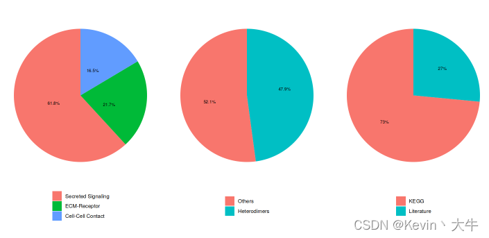
options(repr.plot.height = 7, repr.plot.width = 12)
CellChatDB <- CellChatDB.human
showDatabaseCategory(CellChatDB)
#使用CellChatDB子集进行细胞间通讯分析
CellChatDB.use <- CellChatDB
#若使用全部的数据分析改为：CellChatDB.use <- CellChatDB
#设置使用的数据集在对象中
cellchat@DB <- CellChatDB.use
cellchat <- subsetData(cellchat) #选择信号基因的表达
future::plan("multisession", workers = 4)
cellchat <- identifyOverExpressedGenes(cellchat)
cellchat <- identifyOverExpressedInteractions(cellchat)
cellchat <- projectData(cellchat, PPI.human)

可视化结果如下：

 细胞通信网络的推断

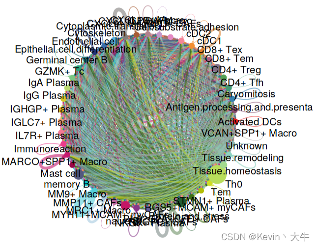
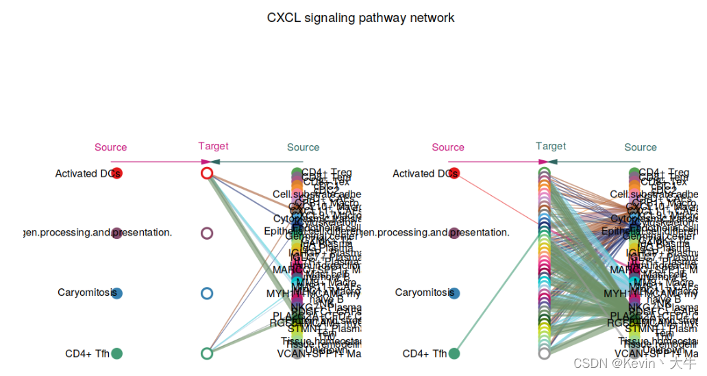
#设置处理最大空间
options(future.globals.maxSize= 3*1024*1024^2) #3*1024MB
cellchat <- computeCommunProb(cellchat, raw.use = TRUE)
#筛选掉特定细胞组中仅少量细胞表达的细胞间通讯
cellchat <- filterCommunication(cellchat, min.cells = 10)
cellchat <- computeCommunProbPathway(cellchat)
cellchat <- aggregateNet(cellchat)
groupSize <- as.numeric(table(cellchat@idents))
options(repr.plot.height = 6, repr.plot.width = 6)
netVisual_circle(cellchat@net$count, vertex.weight = groupSize, weight.scale = T,
                 label.edge= F, title.name = "Number of interactions")
# 细胞通信网络的可视化
#边缘颜色/权重、节点颜色/大小/形状的解释：
#在所有可视化图中，边缘颜色与发送者源一致，边缘权重与交互强度成正比。
#较厚的边缘线表示信号更强。在层次结构图和圆图中，圆的大小与每个细胞组中的细胞数量成正比。
#在层次图中，实心和开放的圆分别代表源和目标。
#在和弦图中，内条颜色表示从相应的外条接收信号的目标。内条大小与目标接收的信号强度成正比。
pathways.show <- c("CXCL") #选择通路
vertex.receiver <- seq(1,4) #细胞群索引
options(repr.plot.height = 9, repr.plot.width = 9)
netVisual_aggregate(cellchat, signaling = pathways.show,
                    vertex.receiver = vertex.receiver, layout = "hierarchy")

可视化结果如下：

 

细胞通信网络系统分析

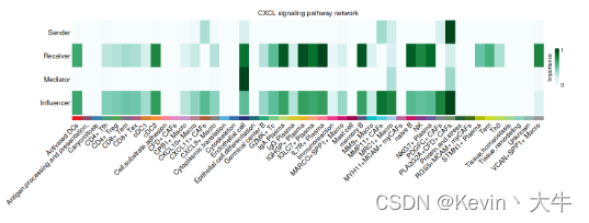
#识别细胞组的信号角色
cellchat <- netAnalysis_computeCentrality(cellchat, slot.name = "netP")
netAnalysis_signalingRole_network(cellchat, signaling = pathways.show, width = 25, height = 5, font.size = 10)

可视化结果如下：

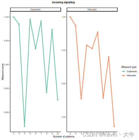
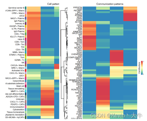
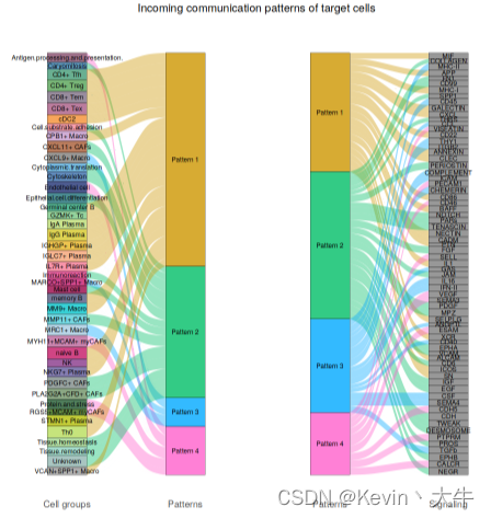
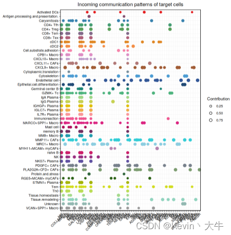
识别和可视化目标细胞的传入通信模式

options(repr.plot.height = 8, repr.plot.width = 8)
selectK(cellchat, pattern = "incoming")
nPatterns = 4
cellchat <- identifyCommunicationPatterns(cellchat, pattern = "incoming", k = nPatterns,
                                          width = 8, height = 18)
netAnalysis_river(cellchat, pattern = "incoming")
netAnalysis_dot(cellchat, pattern = "incoming")

可视化结果如下：

 

 

 

 最后最重要的一步就是把创建的cellchat对象保存下来

saveRDS(cellchat, file = "cellchat_Lymph.RDS")

第二步：比较淋巴结与原发组织细胞间通讯

载入R包并读入数据

library(scibet)
library(Seurat)
library(scater)
library(scran)
library(dplyr)
library(Matrix)
library(cowplot)
library(ggplot2)
library(CellChat)
library(patchwork)
library(harmony)
cellchat.Lymph <- readRDS(file = "cellchat_Lymph.RDS")
cellchat.Primary <- readRDS(file = "cellchat_Primary.RDS")

校正两个数据集的细胞类型有不同

group.new <- levels(cellchat.Primary@idents)
cellchat.Lymph <- liftCellChat(cellchat.Lymph, group.new)

加载数据

object.list <- list(Lymph = cellchat.Lymph, Primary = cellchat.Primary)
cellchat <- mergeCellChat(object.list, add.names = names(object.list))

比较不同细胞群之间的相互作用数量和强度

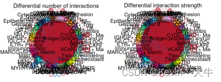
#不同细胞群之间的相互作用数量或强度的差异
par(mfrow = c(1,2), xpd=TRUE)
netVisual_diffInteraction(cellchat, comparison = c(1,2), weight.scale = T)
netVisual_diffInteraction(cellchat, comparison = c(1,2), weight.scale = T, measure = "weight")

可视化结果如下：

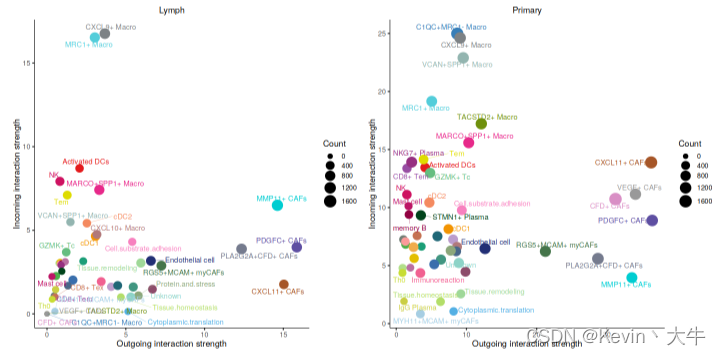
 不同细胞类型之间相互作用或交互强度的差异

options(repr.plot.height = 6, repr.plot.width = 12)
num.link <- sapply(object.list, function(x) {rowSums(x@net$count) + colSums(x@net$count)-diag(x@net$count)})
weight.MinMax <- c(min(num.link), max(num.link)) # control the dot size in the different datasets
gg <- list()
for (i in 1:length(object.list)) {
  gg[[i]] <- netAnalysis_signalingRole_scatter(object.list[[i]], title = names(object.list)[i], weight.MinMax = weight.MinMax)
}
patchwork::wrap_plots(plots = gg)

可视化结果如下：

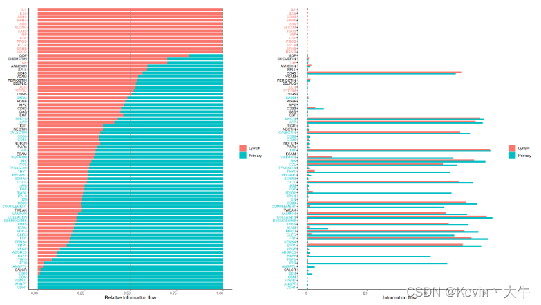
 识别并可视化保守和环境特异的信号通路

#计算和可视化通路距离
options(repr.plot.height = 12, repr.plot.width = 12)
rankSimilarity(cellchat, type = "functional")
#比较每个信号通路的整体信息流
options(repr.plot.height = 10, repr.plot.width = 18)
gg1 <- rankNet(cellchat, mode = "comparison", stacked = T, do.stat = TRUE)
gg2 <- rankNet(cellchat, mode = "comparison", stacked = F, do.stat = TRUE)
gg1 + gg2

可视化结果如下

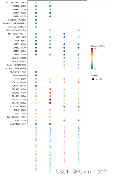
 识别上调和下调的信号配体对

options(repr.plot.height = 10, repr.plot.width = 6)
netVisual_bubble(cellchat, sources.use = c(40), targets.use = c(34,37),  comparison = c(1, 2), angle.x = 90)

可视化结果如下

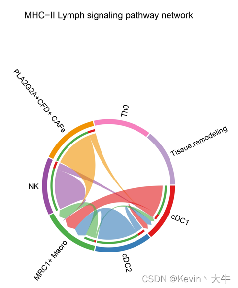
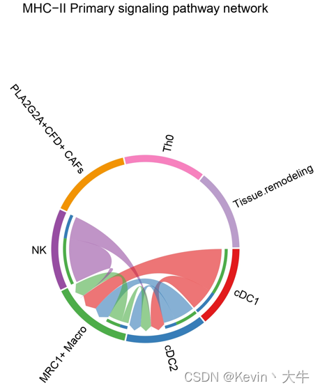
 对细胞间在某通路的互作情况进行网络可视化

p1 <- netVisual_aggregate(object.list.s[[1]], signaling = pathways.show,
                      layout = "chord", signaling.name = paste(pathways.show, names(object.list.s)[1]))
p2 <- netVisual_aggregate(object.list.s[[2]], signaling = pathways.show,
                      layout = "chord", signaling.name = paste(pathways.show, names(object.list.s)[2]))
p1
p2

可视化结果如下

 

 到此我的分析结束，我主要关注的是不同细胞群之间的细胞间通讯在不同组织中有何种差异，当然cellchat可供分析的技术不止于此，大家可以通过自己的渠道再去学习cellchat，希望我的一些经验能够给大家带来一些启发和帮助，也欢迎大家有任何疑问可以一起沟通交流！下一个目标，研究微生物组生物信息学了！单细胞分析就在这里与大家说再见了！