基于PMU的多接地配电系统状态估计研究（Matlab代码实现）

 💥💥💞💞欢迎来到本博客❤️❤️💥💥

🏆博主优势：🌞🌞🌞博客内容尽量做到思维缜密，逻辑清晰，为了方便读者。

⛳️座右铭：行百里者，半于九十。

📋📋📋本文目录如下：🎁🎁🎁

目录

💥1 概述

📚2 运行结果

🎉3 参考文献

🌈4 Matlab代码、数据、文章

---

💥1 概述

摘要：
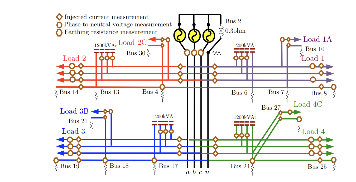
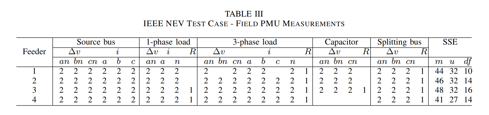
基于线性网络建模和相量测量单元（PMU）简化了传统系统状态估计（SSE）问题。现有的多相SSE-基于PMU模型是线性的，包括接地电阻作为固定和不变的参数。然而，接地电阻在很大程度上取决于时间内的湿度和温度变化。因此，在不平衡运行时，中性接地电压（NEV）可能高于城市地区允许的接触和步进电压。现在可以使用专门的仪表监测接地电阻，并因此在多接地SSE问题中合理地将其作为测量和状态变量加以考虑。因此，SSE问题变得非线性，标准的线性解决方案方法不再适用。这个事实在文献中被忽视了。为了填补研究空白，提出了一种新的基于多接地的SSE-PMU模型。作为一个关键贡献，线性SSE方法中使用的正规方程结构被扩展为非线性结构，以便允许接地电阻、中性对地电压和中性电流的估计。该提议在一个2总线示例中进行了应用以进行说明，并在大规模条件下成功应用和与现有方法进行了比较。系统状态估计是未来电力系统的基石[1]。状态估计器可以为验证传输和配电系统组件模型与现场测量结果提供合适的数学框架。

📚2 运行结果

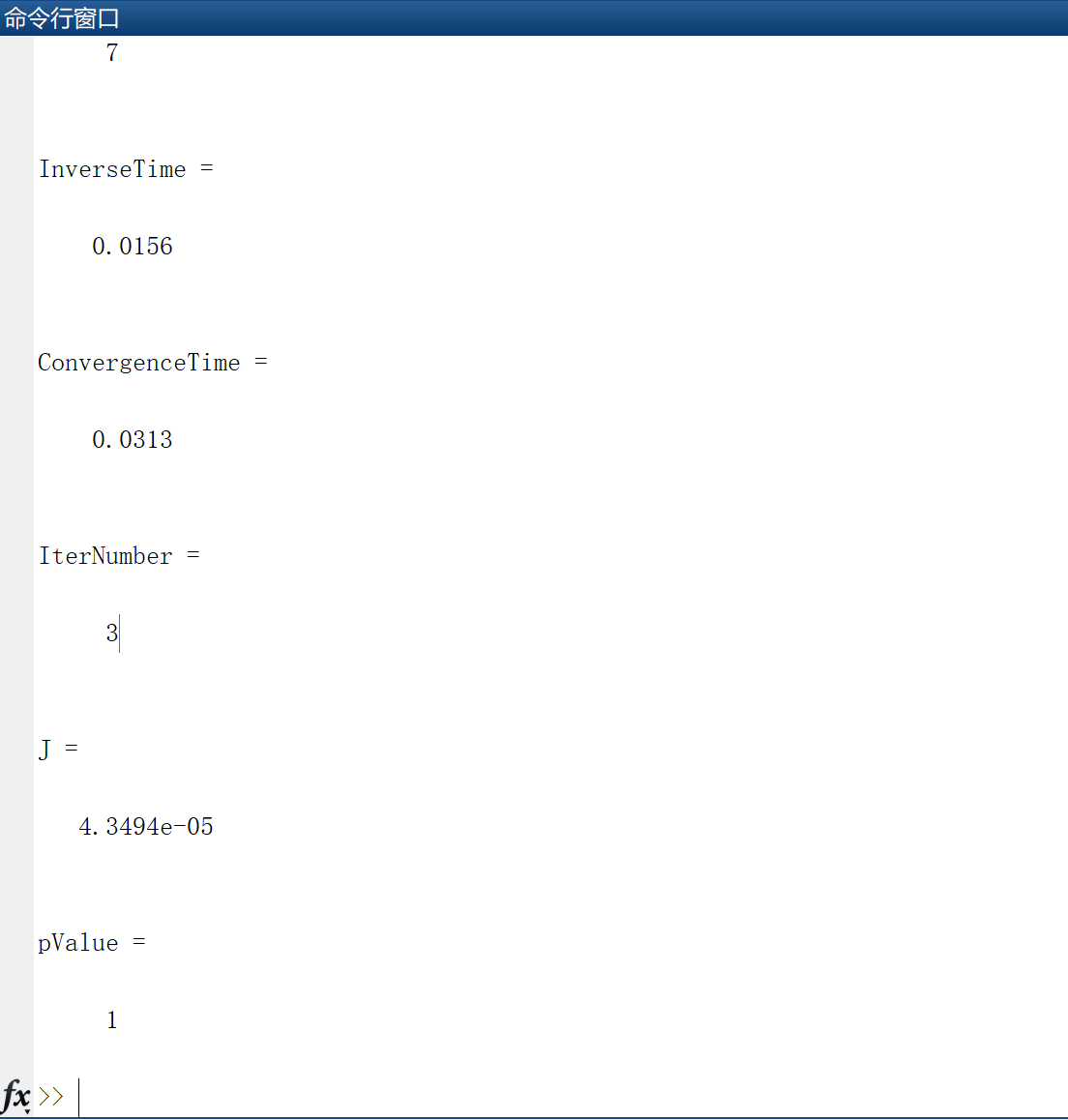
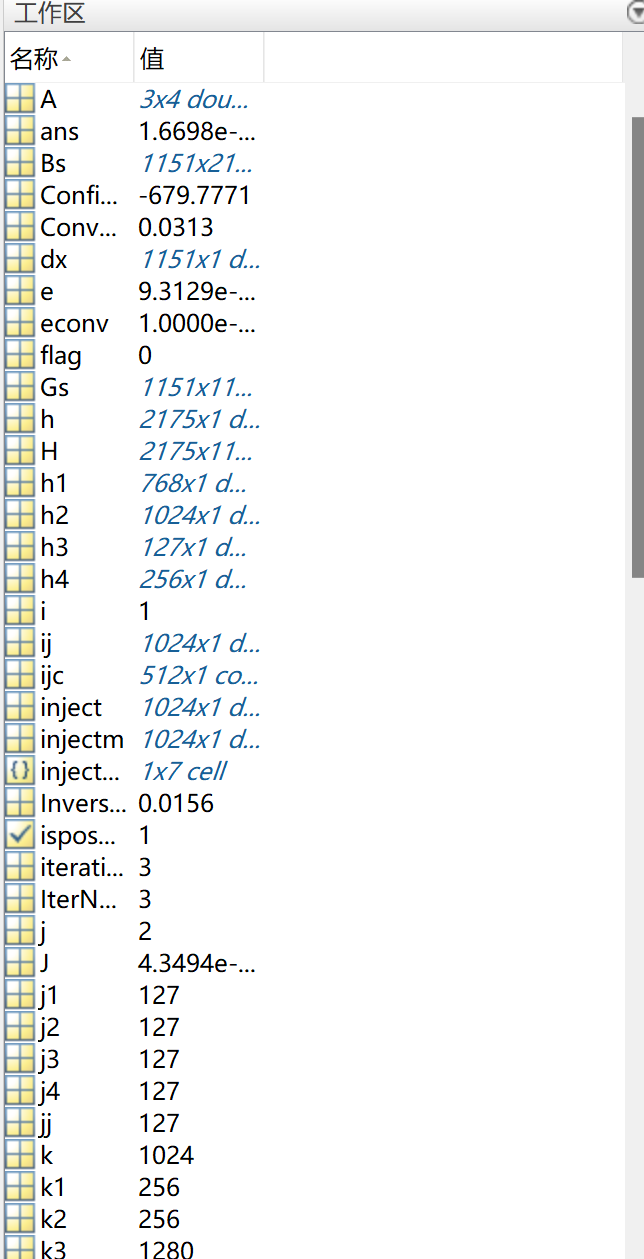
部分代码：

%% General parameters
layer=7  %Choose the number of layers from 1 to 7
nl=.03;%noise level .03=3%
econv=10^-4; %convergence criteria
%% To get 2-bus IEEE Paper Resuls set layer=1
%    layer=1;
%% Runs the  4-wire Power Flow for each layer

%% Begins the iterative process

%% 
ustat=length(Y)+nb-1;% State Vars
m=length(z0);% number of measurements
%% Noise generator, altering the OpenDSS solution zm
lowerbound=-1;
upperbound=1;
for j=1:m
        zalt(j,1)=z0(j,1)*(1+nl*(-lowerbound+(lowerbound+upperbound)*rand(1,1))); 
        %zalt(j,1)=z0(j,1)*(1+nl*unifrnd(lowerbound,upperbound)); 
        %zalt(j,1)=z0(j,1)*(1+nl*normrnd(lowerbound,upperbound));         
end
if layer==1
% Only for l=1 and nl=3% - Paper DSSE example

    kk=kk+1;
zalt(m+kk)=zalt(6*nb+k);
end
%% Meter data accuracy and weights calculation
sigma0=.03;%acuraccy of the meters
SIGMAv0=sigma0*10; %Accuracy (dev stad 1*sigma0% on a scale 10000V)
SIGMAi0=sigma0*.400; %Accuracy (dev stad 1*sigma0% on a scale 400A)
SIGMAin0=sigma0*.100; %Accuracy (dev stad 1*sigma0% on a scale 100A)
SIGMAz0=3*sigma0*5; %Accuracy (dev stad 3*sigma0% on a scale 5 ohm)

%% Kesting NEV Database - Generic n^l bus power flow
a=complex(cos(2*pi/3),sin(2*pi/3));
a2=a^2;
Vo=12.47/sqrt(3);%Nominal voltage kV
Sbase=3;%MVA Base at High Voltage
Vbase=12.47/sqrt(3);%kV base
Ibase=1000*Sbase/Vbase;%Amperes
Zbase=Vbase^2/Sbase;%Zbase high in ohms
f=60;%Frequency Hz
rvd=100; % Resitivity ohm-m
eta=1.6093;%Impedances are Given in ohm/mile
mu0=4*pi*eta/10000;%H/mile
w=2*pi*f;%angular frequency
De=2160*sqrt(rvd/f); %Carson's correction factor 
re=(pi/4)*4*eta*pi*f*0.0001; %Carson's correction ground loop resistance (ohm)
%% DL Data
Length=6000*0.000189393939/(l);%section length in miles
%Length=0.1*60000*0.000189393939/(nb-1);%section length in miles
resist1=0.5;%ohms
resist2=5.0;%ohms
GMRf=0.0244;%feet phase
rf=1*0.306;%ohm/mile
GMRn=0.00814;%feet
rn=1*0.5920;%ohm/mile neutral
%Spacings
Dab=2.5;%feet
Dbc=4.5;%feet
Dac=Dab+Dbc;%feet
Dcn=(4*4+3*3)^.5;%feet
Dbn=(4*4+1.5*1.5)^.5;%feet

🎉3 参考文献

文章中一些内容引自网络，会注明出处或引用为参考文献，难免有未尽之处，如有不妥，请随时联系删除。

[1]Paulo M. De Oliveira-De Jesus, Nelson A. Rodriguez, David F. Celeita , Gustavo A. Ramos (2020) PMU-Based System State Estimation for Multigrounded Distribution Systems 

🌈4 Matlab代码、数据、文章