3D Gaussian Splatting——配置与实例

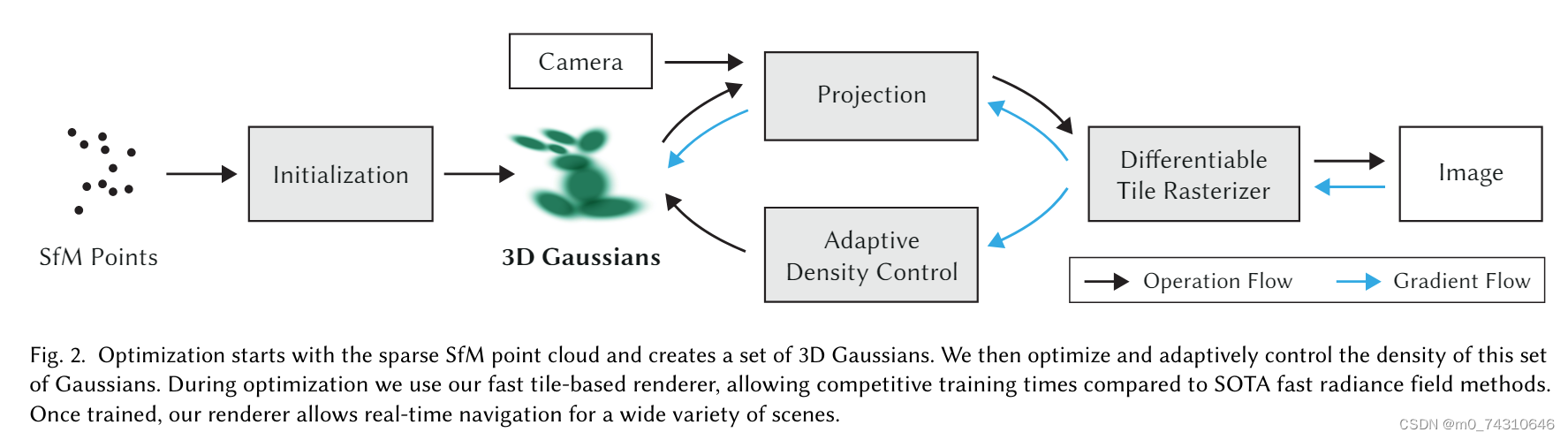
3DGS是目前三维重建领域中的大作和经典之作，原理相信有很多人介绍过了，原理篇会在后面有空的时候更新，这里只做实例讲解。事实上，3DGS做了这样一件事情：首先输入一个稀疏的点云（一般是利用colmap的经典稀疏重建方法得到）相比于神经辐射场NeRF，3DGS不对每根光线做建模以及采样点的神经网络计算（太耗费内存与计算资源），他将每一个点建模为一个椭球（高斯分布），具体地，每一个高斯分布的参数涉及协方差，而这个协方差之列向量正好可以看作是旋转平移变换！

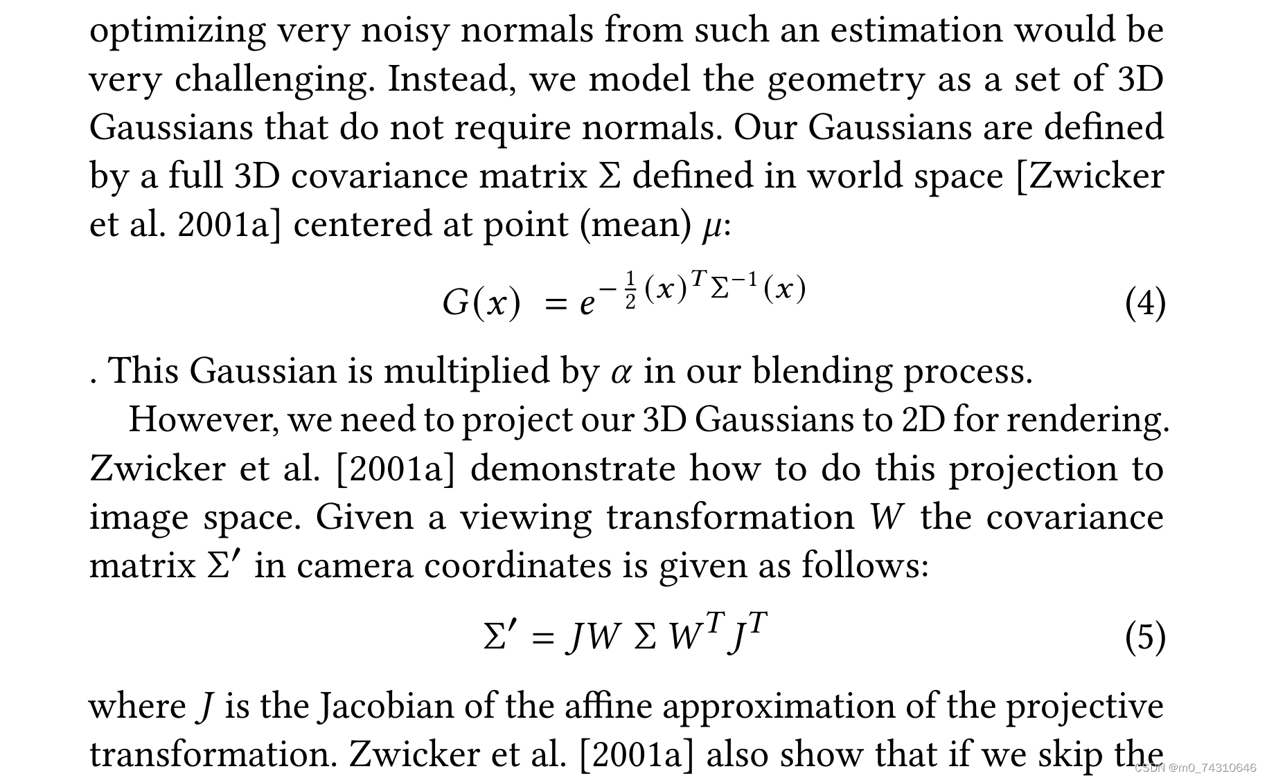
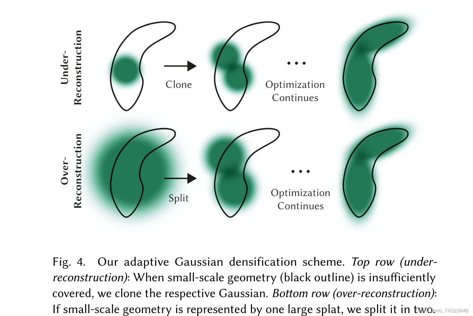
然后，就是这个Splatting过程，对于任意的点，会经过分裂或者clone的过程，得到一个稠密点云，然后渲染（注意这个渲染叫可微光栅化，与NeRF对于每条光线采样建模不一样）得到估计的图像，与原始图像做loss，以调整里面的各个参数。我们可以发现，3DGS是一个显式建模的过程，即可以看作是由一个几百万（这个数字是建模以后得到的）个高斯分布组成的庞大的高斯群（字面意思，非数学中的群），而NeRF对于场景的建模则是一个MLP！

3DGS在很多方面优于NeRF，比如训练速度，渲染速度，建模场景等，NeRF的优势在于，它可以表示连续的高分辨的场景，并且可以转成mesh来使用，而3DGS转mesh一直是一个令人头疼的问题，正如valse2024的workshop中学者方杰民所表达的，对于3DGS来说，consistency与geometry是一个trade-off。

1.先从官网开始配置环境

放上原作的code链接：

GitHub - graphdeco-inria/gaussian-splatting: Original reference implementation of "3D Gaussian Splatting for Real-Time Radiance Field Rendering"Original reference implementation of "3D Gaussian Splatting for Real-Time Radiance Field Rendering" - graphdeco-inria/gaussian-splattinghttps://github.com/graphdeco-inria/gaussian-splatting按照这个提示基本不会报错：

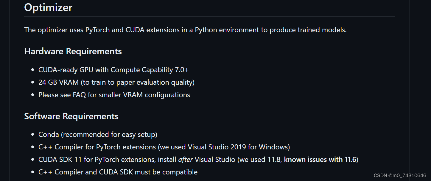
大概的配置要求，但是后面train.py中有低配的参数配置

（1）clone

Cloning the Repository
The repository contains submodules, thus please check it out with

# SSH
git clone git@github.com:graphdeco-inria/gaussian-splatting.git --recursive
or

# HTTPS
git clone https://github.com/graphdeco-inria/gaussian-splatting --recursive

（2）配置环境

Setup
Local Setup
Our default, provided install method is based on Conda package and environment management:

SET DISTUTILS_USE_SDK=1 # Windows only
conda env create --file environment.yml
conda activate gaussian_splatting
Please note that this process assumes that you have CUDA SDK 11 installed, not 12. For modifications, see below.

Tip: Downloading packages and creating a new environment with Conda can require a significant amount of disk space. By default, Conda will use the main system hard drive. You can avoid this by specifying a different package download location and an environment on a different drive:

conda config --add pkgs_dirs <Drive>/<pkg_path>
conda env create --file environment.yml --prefix <Drive>/<env_path>/gaussian_splatting
conda activate <Drive>/<env_path>/gaussian_splatting

2.开始上手训练

2.1数据的预处理——从图片到稀疏点云

3DGS的输入是一个稀疏点云，这需要将数据集的图片转为稀疏点云，一般使用colmap，关于colmap的使用可以看我的另一篇：

一份colmap tutorial的阅读笔记（更新中）——Windows版本_colmap在windows怎么用-CSDN博客https://blog.csdn.net/m0_74310646/article/details/137889450?spm=1001.2014.3001.5501这里，作者在代码中提供了预处理.py文件，就是convert.py，里面有colmap的处理参数和命令，直接用这个脚本执行即可得到稀疏点云。

这里我自己根据里面的代码，重新手动运行了整个过程，数据使用的是colmap官网提供的数据集，大家可以去自行下载。

需要注意的是，对于文件夹路径，一定要根据convert.py来创建，否则后面执行train.py会因为路径问题报错！！！找路径哪里有问题还是很麻烦的。

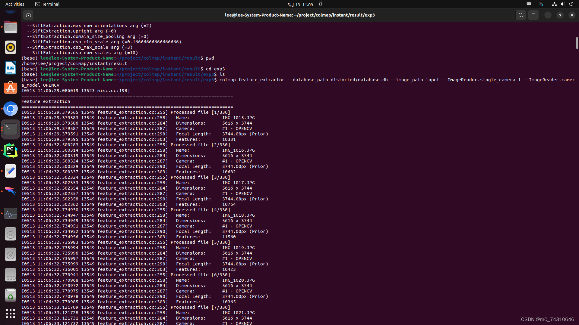
（1）特征提取——参数全是来自convert.py

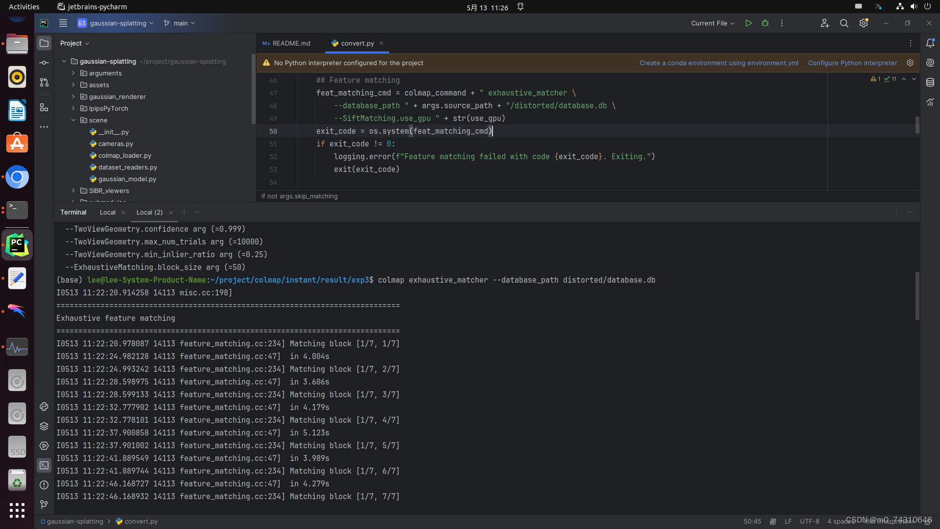
（2）特征匹配——上面是convert.py，下面是对应的手动命令，convert.py中默认了exhaustive matching，如果图片数量很多的话推荐使用其他匹配算法，具体的使用可以看我那篇文章。

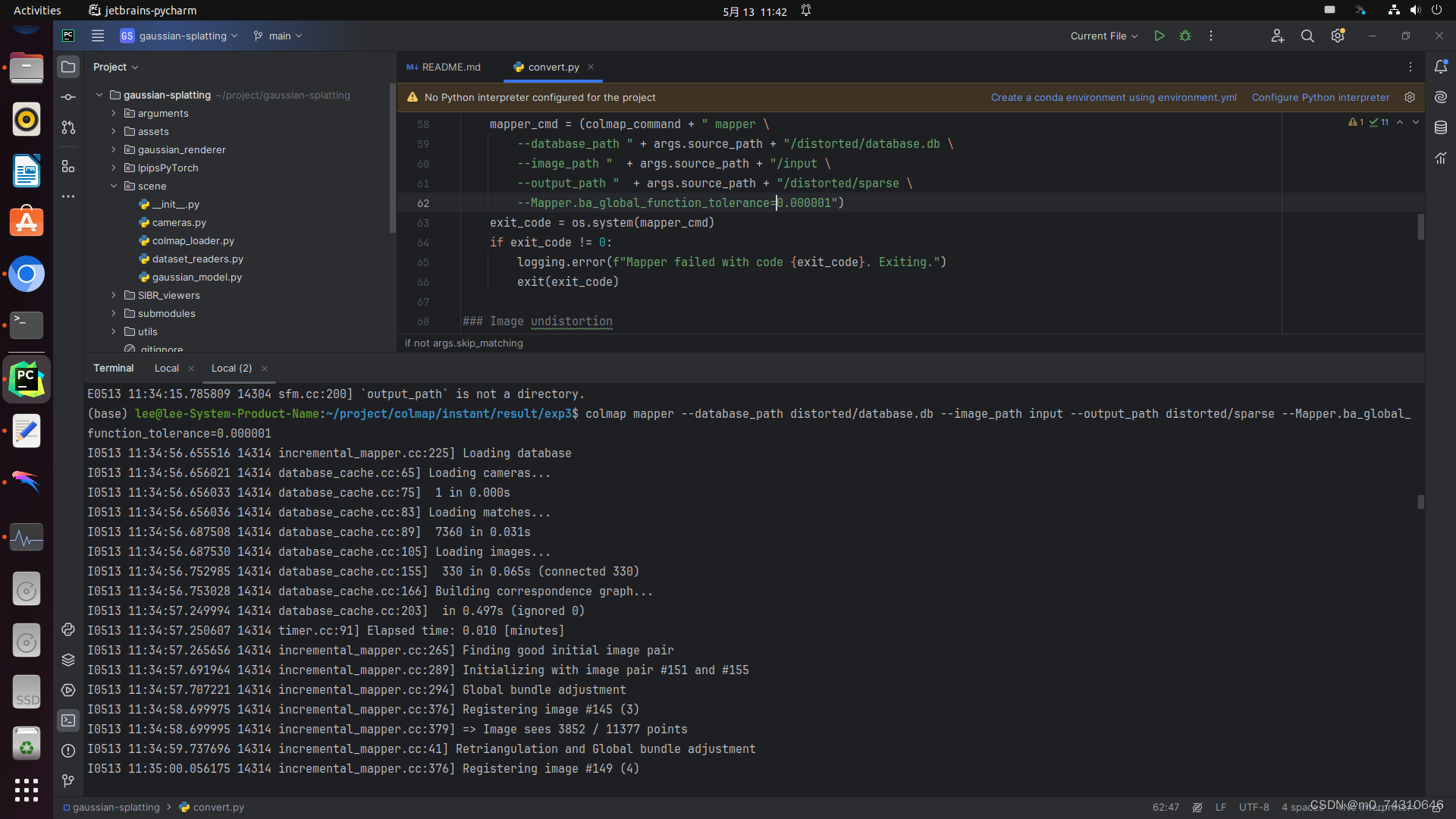
（3）稀疏重建——mapper

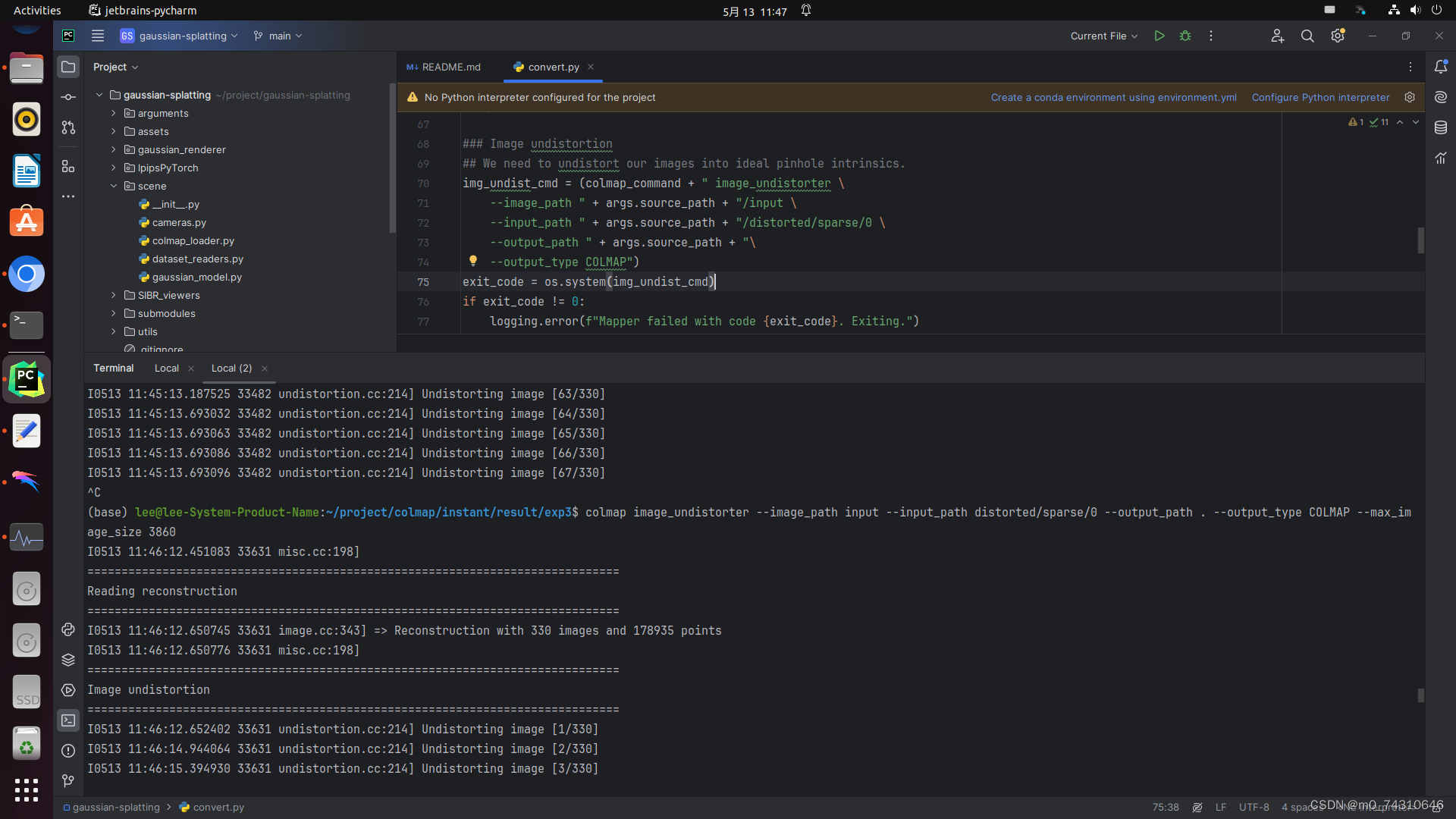
（4）去畸变

（5）转换稀疏点云格式——注意稀疏点云的路径

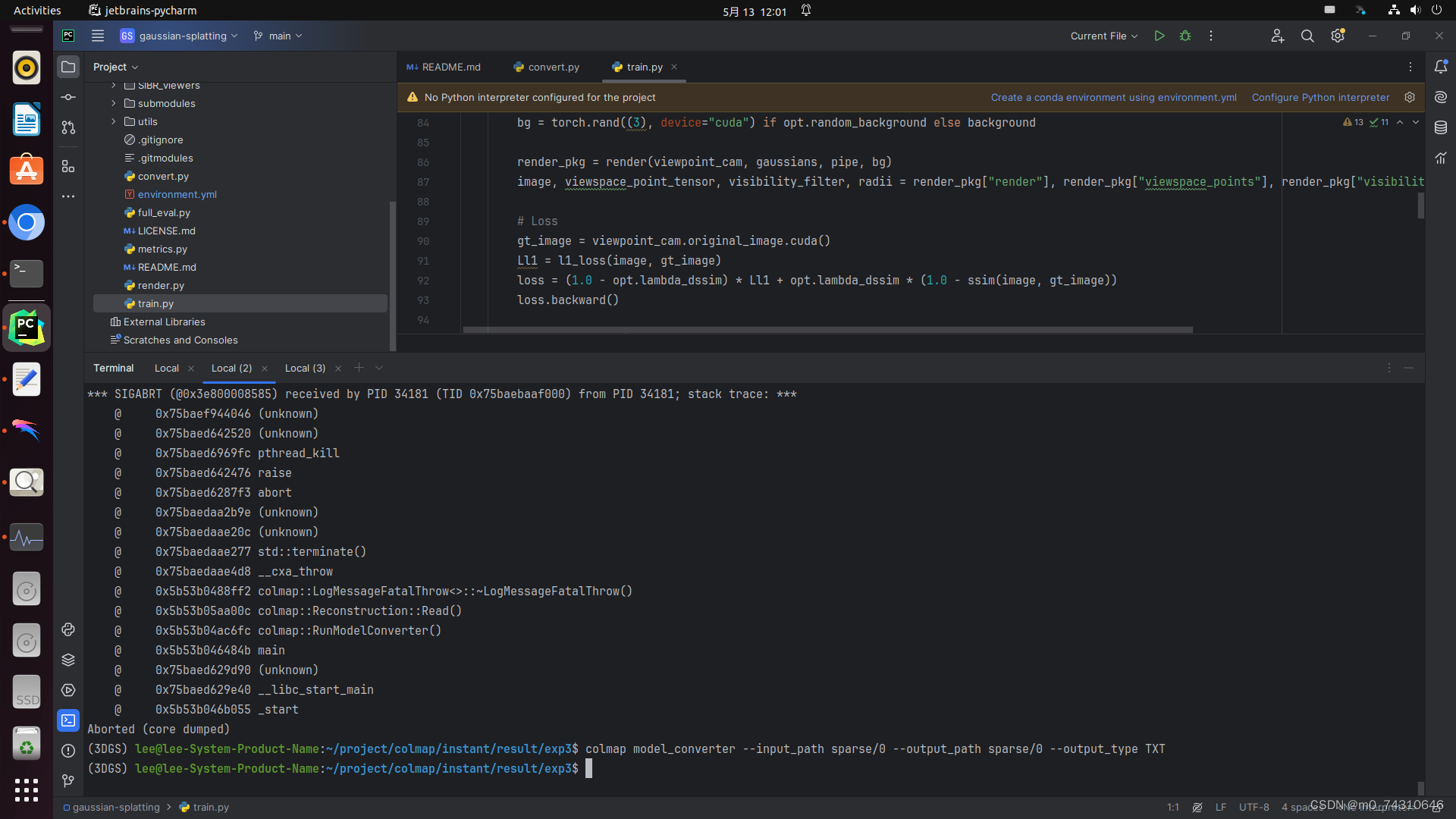
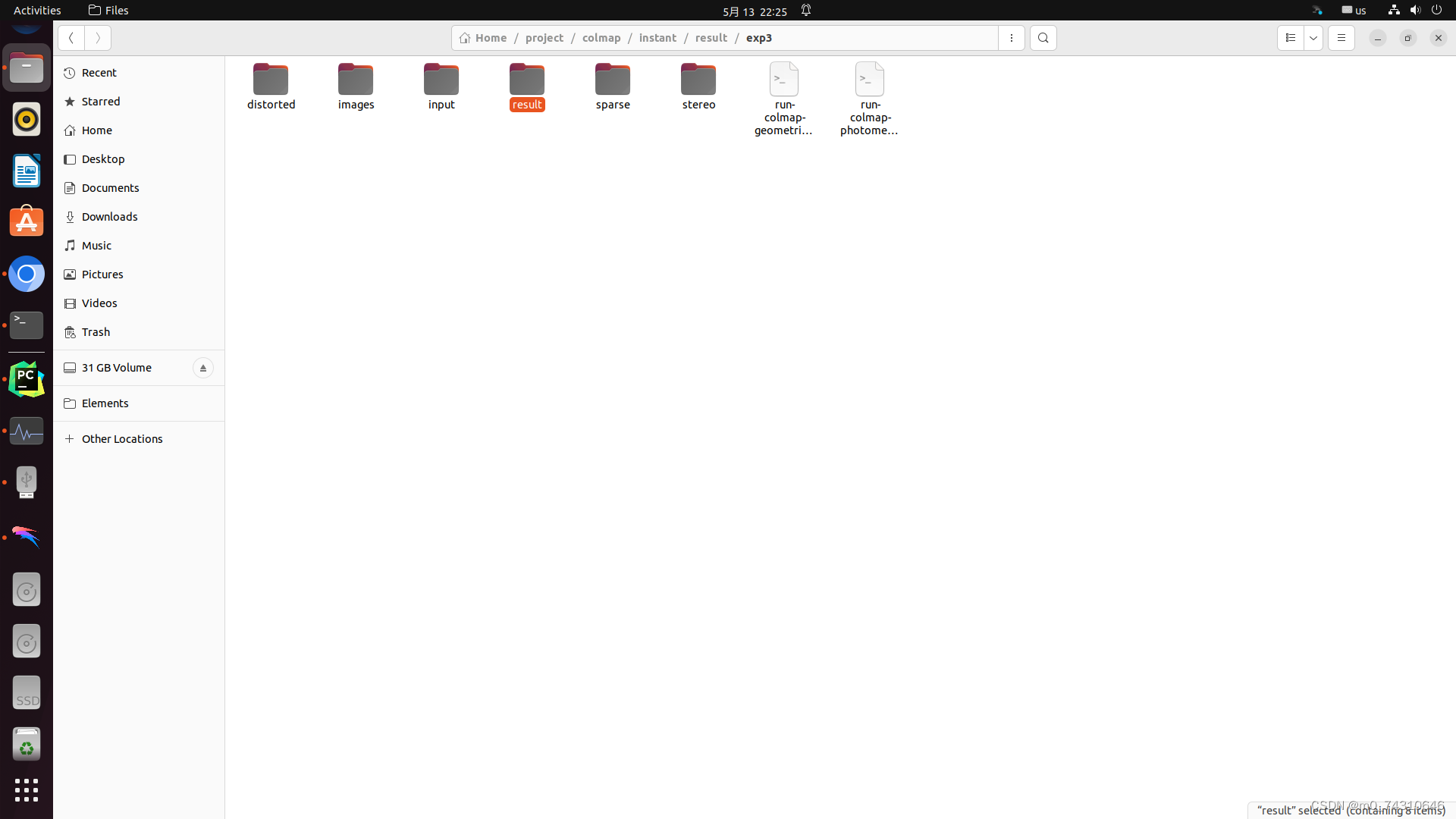
（6）完成以后，路径中长这样，result除外，是我自己建的模型输出路径

2.2 训练

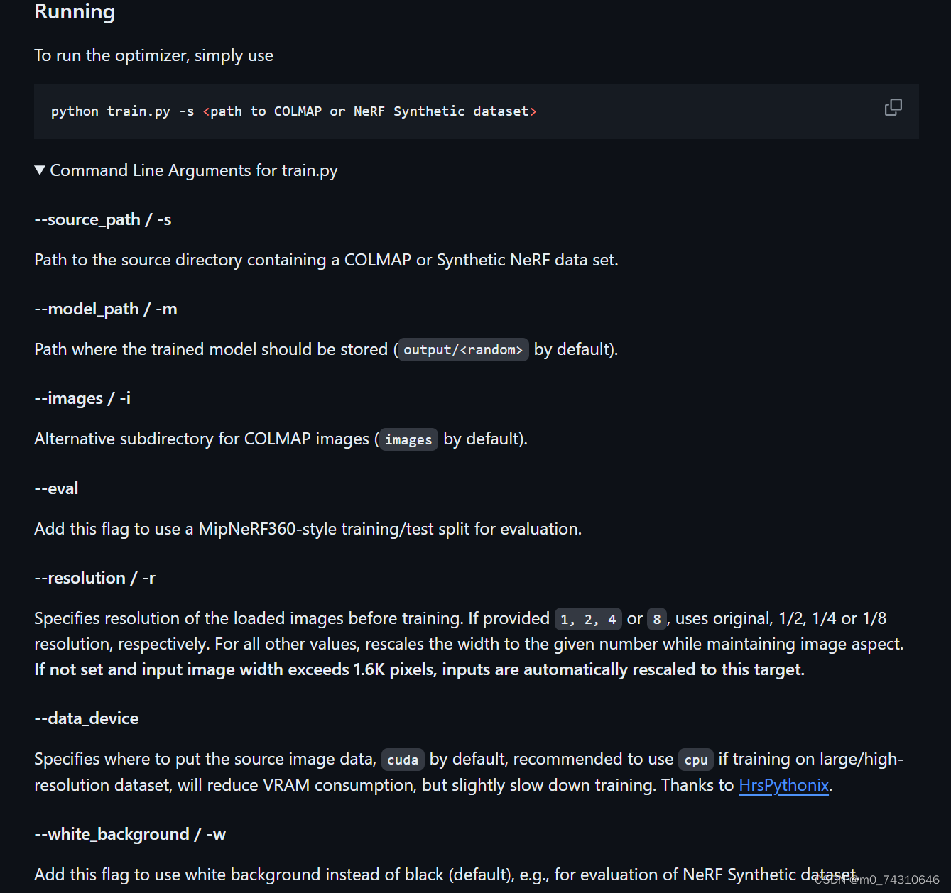
官网的命令很简单，一堆参数默认即可：

python train.py -s <path to COLMAP or NeRF Synthetic dataset>

对于参数，可以通过python train.py -h来查看

在这里我使用的参数也不多：

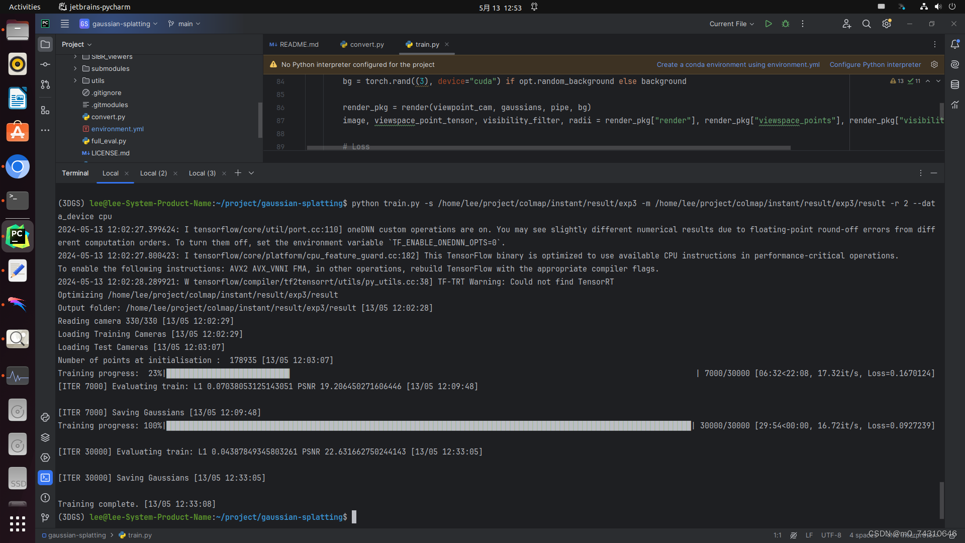
训练出来的psnr在22左右，有点低，应该是还需要调整其他参数，这里iteration默认设置为30000，一般来说，iteration是图片数量的60-100倍左右，我的图片数量在330张。下面附上train相关的参数，训练比较重要，着重介绍

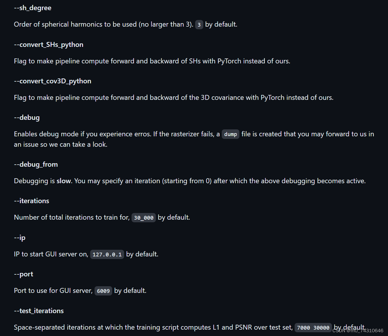
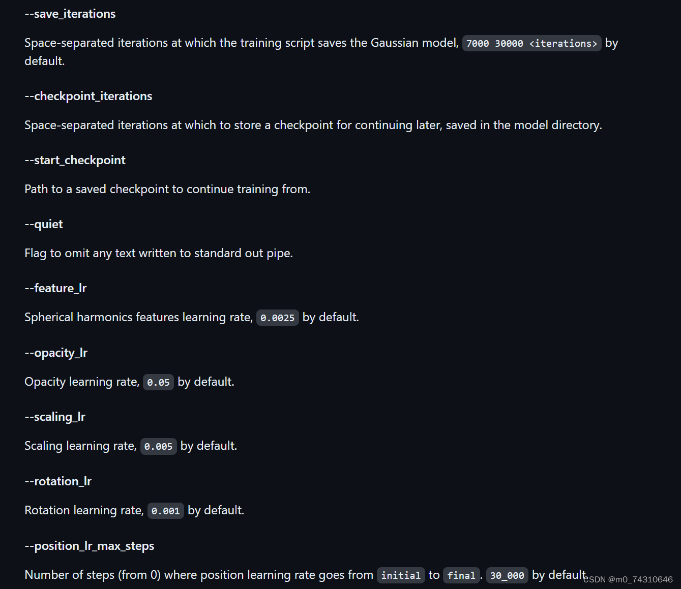
小经验：

-s是source路径，就是创建项目的目录，例如这个/exp3就是source路径

-m是输出模型的路径

-r是分辨率，2会降低到一半，4是1/4，，，因为分辨率太高容易爆显存OOM，或者电脑内存爆炸死机！

--data device cpu可以降低显存占用，避免显存不足

-iteration一般是图片数量的60-100倍左右

2.3Evaluation

这里是严格的实验过程，直接参考官网即可，render.py，metric.py都有具体的参数，可以根据具体任务来查看

By default, the trained models use all available images in the dataset. To train them while withholding a test set for evaluation, use the --eval flag. This way, you can render training/test sets and produce error metrics as follows:

python train.py -s <path to COLMAP or NeRF Synthetic dataset> --eval # Train with train/test split
python render.py -m <path to trained model> # Generate renderings
python metrics.py -m <path to trained model> # Compute error metrics on renderings
If you want to evaluate our pre-trained models, you will have to download the corresponding source data sets and indicate their location to render.py with an additional --source_path/-s flag. Note: The pre-trained models were created with the release codebase. This code base has been cleaned up and includes bugfixes, hence the metrics you get from evaluating them will differ from those in the paper.

python render.py -m <path to pre-trained model> -s <path to COLMAP dataset>
python metrics.py -m <path to pre-trained model>

依照比例划分训练集与测试集，在执行metres.py之前，需要先render.py渲染出测试集上的图像，然后再执行metres.py与原数据对比计算。具体地，还能在训练过程中完成划分训练集与测试集，与固定iteration点上完成测试，计算psnr，这些参数可以查看train.py的参数

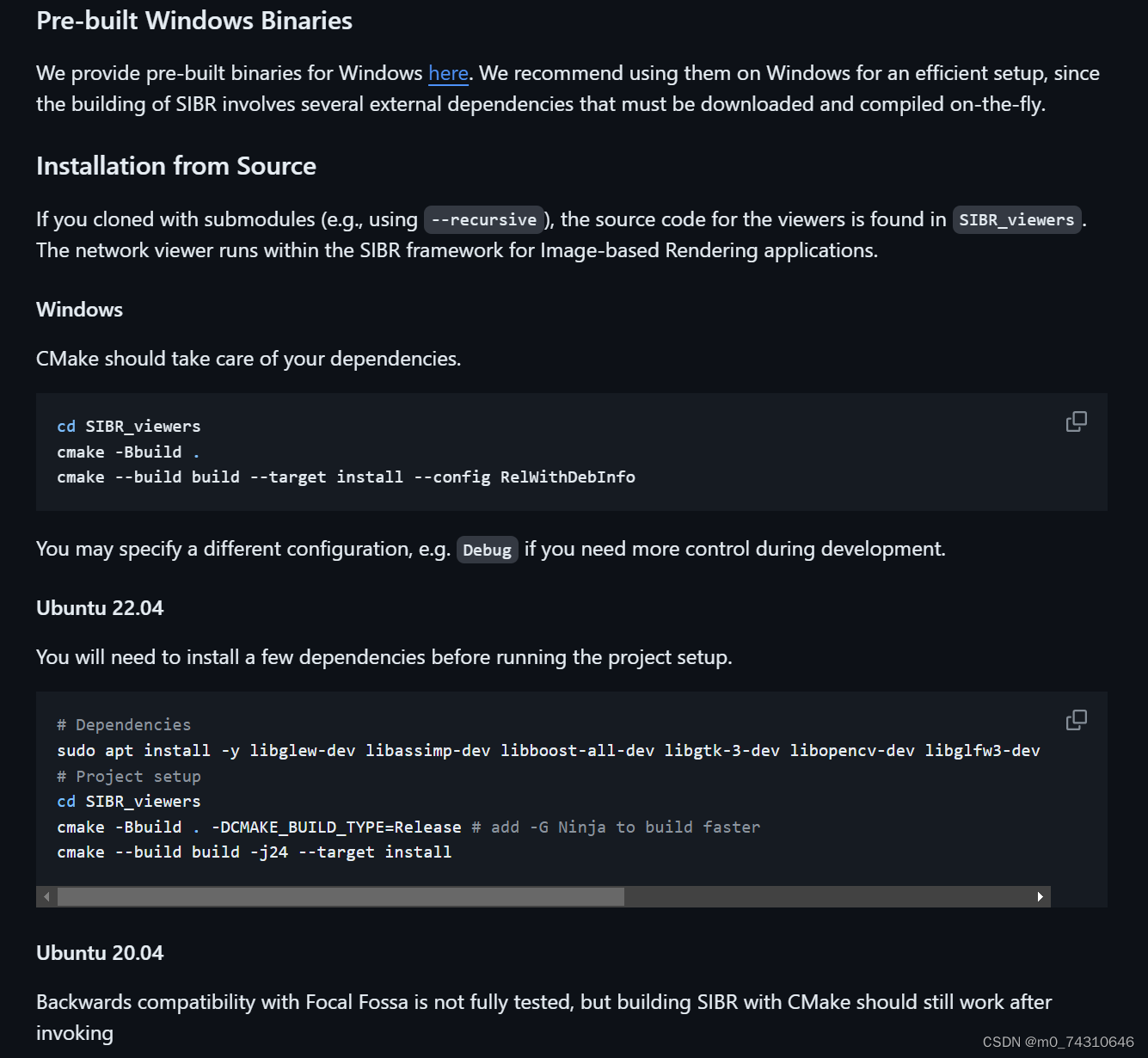
3.viewer——SIBR

3.1编译

SIBR首先需要编译，这个过程也基本不会报错，就是会稍微有点久：

3.2使用

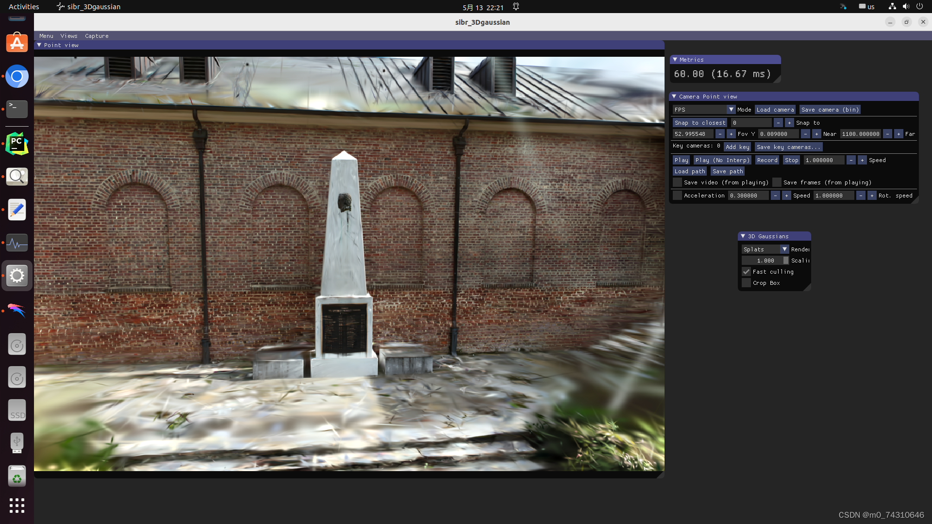
SIBR可以实时查看训练过程中高斯球的变换过程：

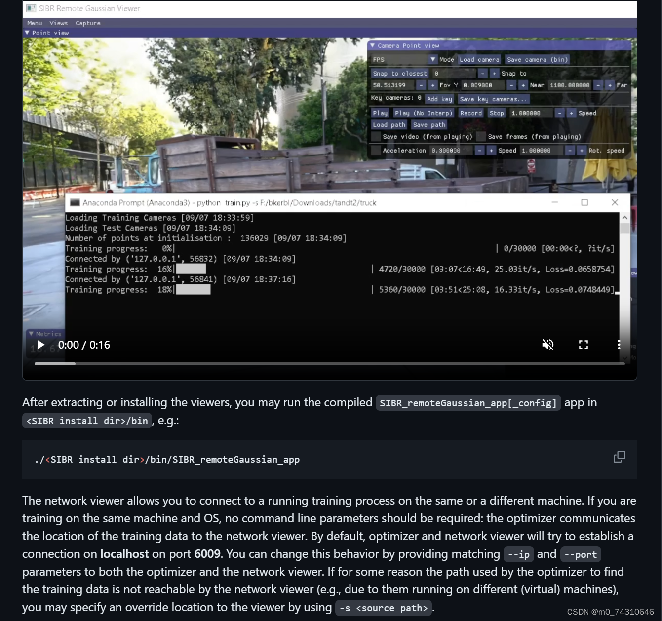
对于训练好的模型，直接用下面的命令即可查看，注意最前面那个点，否则会报错

下面是我的命令执行，我的模型放在这个位置：

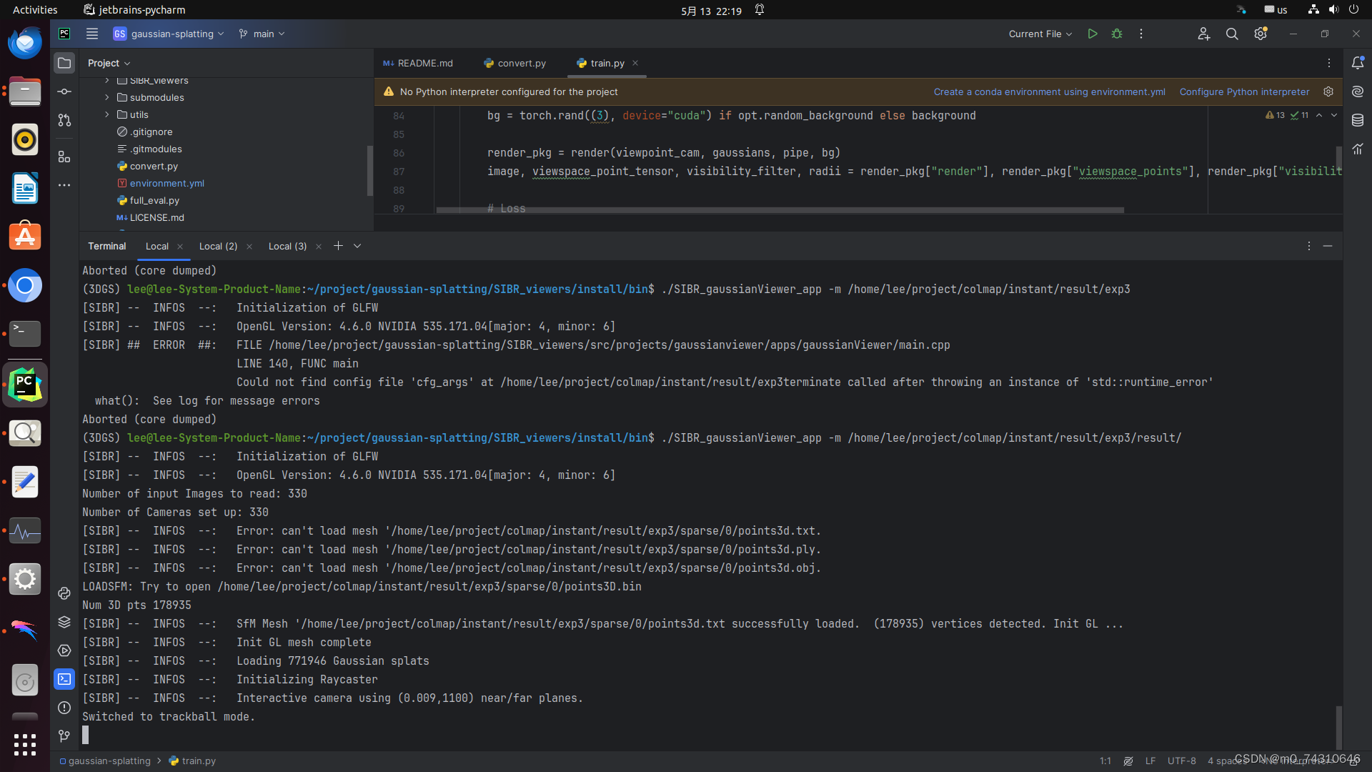
./SIBR_gaussianViewer_app -m /home/lee/project/colmap/instant/result/exp3/result

3.3查看

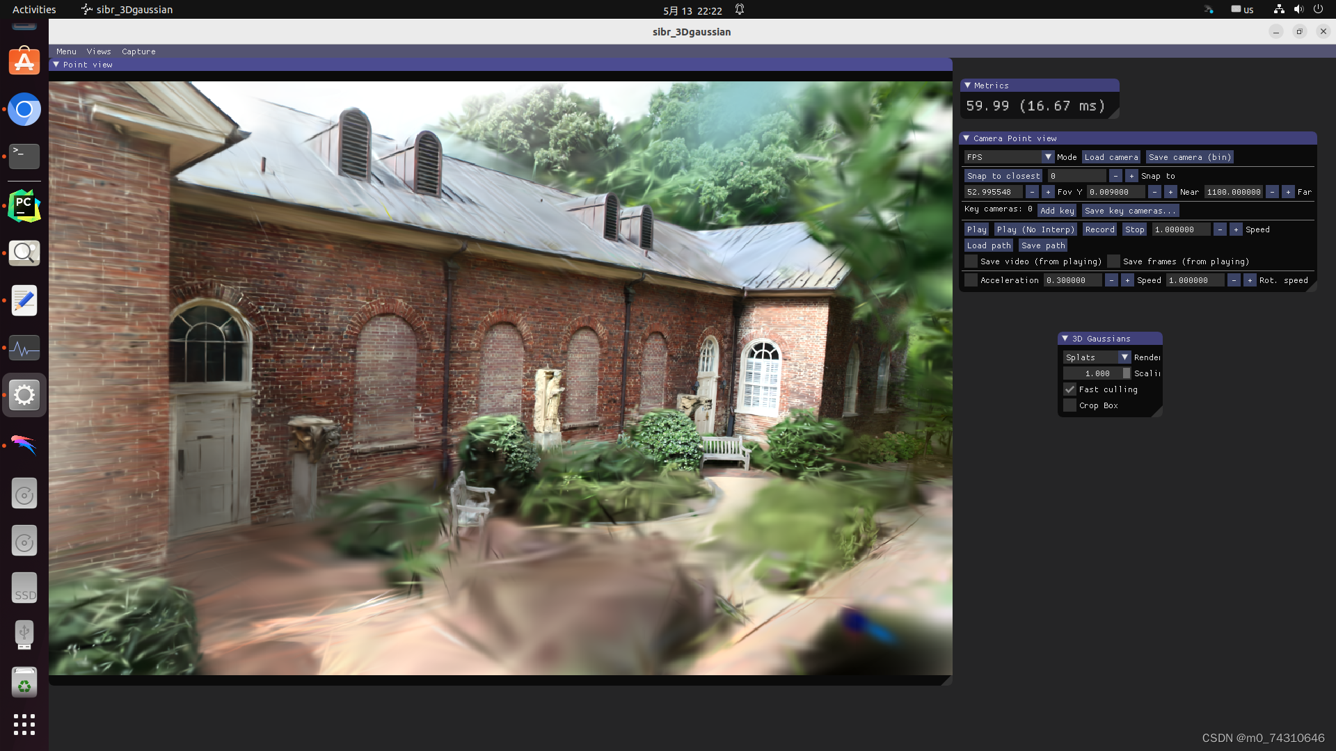
查看点云：