论文翻译《Toward Multimodal Image-to-Image Translation》

论文地址：https://arxiv.org/abs/1711.11586
代码地址：https://github.com/junyanz/BicycleGAN

Abstract

Many image-to-image translation problems are ambiguous, as a single input image may correspond to multiple possible outputs. In this work, we aim to model a distribution of possible outputs in a conditional generative modeling setting. The ambiguity of the mapping is distilled in a low-dimensional latent vector, which can be randomly sampled at test time. A generator learns to map the given input, combined with this latent code, to the output. We explicitly encourage the connection between output and the latent code to be invertible. This helps prevent a many-to-one mapping from the latent code to the output during training, also known as the problem of mode collapse, and produces more diverse results. We explore several variants of this approach by employing different training objectives, network architectures, and methods of injecting the latent code. Our proposed method encourages bijective consistency between the latent encoding and output modes. We present a systematic comparison of our method and other variants on both perceptual realism and diversity.

许多图像到图像的转换问题是模糊的，因为单个输入图像可能对应多个可能的输出。在这项工作中，我们的目标是在条件生成建模设置中对可能输出的分布进行建模。映射的模糊性被提取到一个低维的隐向量中，该隐向量可以在测试时随机采样。生成器学习将给定的输入与隐代码相结合，映射到输出。我们明确地鼓励输出和隐代码之间的连接是可逆的。这有助于防止在训练期间从隐代码到输出的多对一映射，也称为模式崩溃问题，并产生更多样化的结果。我们通过使用不同的训练目标、网络架构和注入隐代码的方法来探索这种方法的几种变体。我们提出的方法鼓励隐码和输出模式之间的客观一致性。我们对我们的方法和其他变体在感知真实性和多样性方面进行了系统比较。

1 Introduction

Deep learning techniques have made rapid progress in conditional image generation. For example, networks have been used to inpaint missing image regions [20, 34, 47], add color to grayscale images [19, 20, 27, 50], and generate photorealistic images from sketches [20, 40]. However, most techniques in this space have focused on generating a single result. In this work, we model a distribution of potential results, as many of these problems may be multimodal in nature. For example, as seen in Figure 1, an image captured at night may look very different in the day, depending on cloud patterns and lighting conditions. We pursue two main goals: producing results which are (1) perceptually realistic and (2) diverse, all while remaining faithful to the input.

深度学习技术在条件图像生成方面进展迅速。例如，网络已被用于为缺失的图像区域上色[20, 34, 47]，为灰度图像添加颜色[19, 20, 27, 50]，以及从草图生成逼真的图像[20, 40]。然而，这一领域的大多数技术都侧重于生成单个结果。在这项工作中，我们对潜在结果的分布进行了建模，因为这些问题中的许多在本质上可能是多模态的。例如，如图 1 所示，根据云层模式和光照条件的不同，夜间拍摄的图像在白天看起来可能截然不同。我们追求两个主要目标：生成 (1) 真实的感知结果和 (2) 多样的结果，同时保持对输入的忠实。

Mapping from a high-dimensional input to a high-dimensional output distribution is challenging. A common approach to representing multimodality is learning a low-dimensional latent code, which should represent aspects of the possible outputs not contained in the input image. At inference time, a deterministic generator uses the input image, along with stochastically sampled latent codes, to produce randomly sampled outputs. A common problem in existing methods is mode collapse [14], where only a small number of real samples get represented in the output. We systematically study a family of solutions to this problem.

从高维输入到高维输出分布的映射具有挑战性。表示多模态的一种常用方法是学习低维隐代码，它应该表示输入图像中不包含的可能输出的各个方面。在推理时，确定性生成器使用输入图像以及随机采样的隐代码来产生随机采样的输出。现有方法的一个常见问题是模式坍塌[14]，即只有少量真实样本在输出中得到表示。我们系统地研究了这一问题的一系列解决方案。

We start with the pix2pix framework [20], which has previously been shown to produce highquality results for various image-to-image translation tasks. The method trains a generator network, conditioned on the input image, with two losses: (1) a regression loss to produce similar output to the known paired ground truth image and (2) a learned discriminator loss to encourage realism. The authors note that trivially appending a randomly drawn latent code did not produce diverse results. Instead, we propose encouraging a bijection between the output and latent space. We not only perform the direct task of mapping the latent code (along with the input) to the output but also jointly learn an encoder from the output back to the latent space. This discourages two different latent codes from generating the same output (non-injective mapping). During training, the learned encoder attempts to pass enough information to the generator to resolve any ambiguities regarding the output mode. For example, when generating a day image from a night image, the latent vector may encode information about the sky color, lighting effects on the ground, and cloud patterns. Composing the encoder and generator sequentially should result in the same image being recovered. The opposite should produce the same latent code.

我们首先使用 pix2pix 框架 [20]，该框架之前已被证明能为各种图像到图像的转换任务提供高质量的结果。该方法以输入图像为条件训练一个生成器网络，有两个损失：(1) 一个回归损失，以产生与已知的配对ground-truth图像相似的输出；(2) 一个学习的判别器损失，以鼓励真实感。作者指出，简单地添加随机的隐代码并不能产生不同的结果。相反，我们建议鼓励在输出和隐空间之间建立双向映射。我们不仅要完成将隐代码（连同输入）映射到输出的直接任务，还要联合学习一个从输出返回到隐空间的编码器。这就避免了两个不同的隐码产生相同的输出（非注入式映射）。在训练过程中，学习的编码器尝试将足够的信息传递给生成器，以解决有关输出模式的任何歧义。例如，当从夜间图像生成白天图像时，隐向量可能会编码有关天空颜色、地面光照效果和云层模式的信息。将编码器和生成器按顺序组合，应能恢复出同一幅图像。相反的应该产生相同的隐代码。

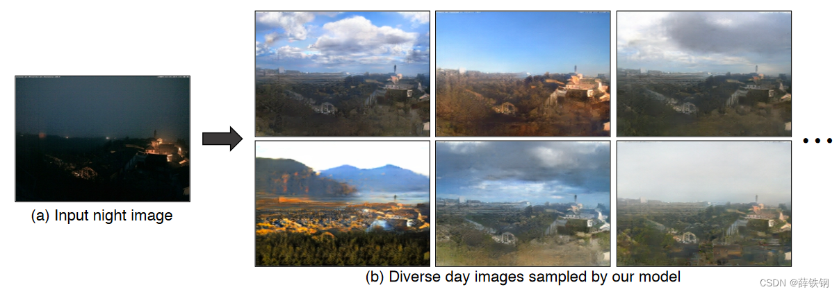
Figure 1: Multimodal image-to-image translation using our proposed method: given an input image from one domain (night image of a scene), we aim to model a distribution of potential outputs in the target domain (corresponding day images), producing both realistic and diverse results.

图 1：使用我们提出的方法进行多模态图像到图像的转换：给定一个域（场景的夜间图像）的输入图像，我们的目标是模拟目标域（相应的白天图像）的潜在输出分布，从而产生既真实又多样化的结果。

In this work, we instantiate this idea by exploring several objective functions, inspired by literature in unconditional generative modeling:

在这项工作中，我们通过探索几个目标函数来实例化这个想法，灵感来自于无条件生成建模中的文献：

1、cVAE-GAN (Conditional Variational Autoencoder GAN): One approach is first encoding the ground truth image into the latent space, giving the generator a noisy “peek" into the desired output. Using this, along with the input image, the generator should be able to reconstruct the specific output image. To ensure that random sampling can be used during inference time, the latent distribution is regularized using KL-divergence to be close to a standard normal distribution. This approach has been popularized in the unconditional setting by VAEs [23] and VAE-GANs [26].

1、cVAE-GAN (条件变分自编码器GAN)：一种方法是首先将真实图像编码到隐空间中，让生成器对期望的输出进行有噪声的“窥视”。利用这一点，加上输入图像，生成器应该能够重建特定的输出图像。为了确保在推理时间内可以使用随机采样，使用KL-散度对潜在分布进行正则化，使其接近标准正态分布。该方法已被VAEs [ 23 ]和VAE-GANs [ 26 ]推广到无条件环境中。

2、cLR-GAN (Conditional Latent Regressor GAN): Another approach is to first provide a randomly drawn latent vector to the generator. In this case, the produced output may not necessarily look like the ground truth image, but it should look realistic. An encoder then attempts to recover the latent vector from the output image. This method could be seen as a conditional formulation of the “latent regressor" model [8, 10] and also related to InfoGAN [4].

2、cLR-GAN(条件潜在回归器GAN)：另一种方法是首先向生成器提供随机生成的隐向量。在这种情况下，生成的输出可能不一定看起来像ground-truth图像，但它应该看起来很逼真。然后编码器尝试从输出图像中恢复隐向量。这种方法可以看作是"隐回归"模型[8、10]的一个条件形式，也与InfoGAN有关[4]。

3、BicycleGAN: Finally, we combine both these approaches to enforce the connection between latent encoding and output in both directions jointly and achieve improved performance. We show that our method can produce both diverse and visually appealing results across a wide range of imageto-image translation problems, significantly more diverse than other baselines, including naively adding noise in the pix2pix framework. In addition to the loss function, we study the performance with respect to several encoder networks, as well as different ways of injecting the latent code into the generator network.

3、BicycleGAN：最后，我们将这两种方法结合起来，在两个方向上共同加强隐代码和输出之间的联系，从而提高了性能。我们表明，我们的方法可以在广泛的图像到图像的转换问题中产生多样化和视觉上吸引人的结果，比其他基线更多样化，包括在pix2pix框架中简单地添加噪声。除了损失函数外，我们还研究了几种编码器网络的性能，以及将隐代码注入生成器网络的不同方法。

We perform a systematic evaluation of these variants by using humans to judge photorealism and a perceptual distance metric [52] to assess output diversity. Code and data are available at https: //github.com/junyanz/BicycleGAN.

我们通过人类判断真实感和感知距离度量[52]来评估输出多样性，对这些变体进行了系统评估。代码和数据可从https://github.com/junyanz/BicycleGAN获得。

2 Related Work

Generative modeling Parametric modeling of the natural image distribution is a challenging problem. Classically, this problem has been tackled using restricted Boltzmann machines [41] and autoencoders [18, 43]. Variational autoencoders [23] provide an effective approach for modeling stochasticity within the network by reparametrization of a latent distribution at training time. A different approach is autoregressive models [11, 32, 33], which are effective at modeling natural image statistics but are slow at inference time due to their sequential predictive nature. Generative adversarial networks [15] overcome this issue by mapping random values from an easy-to-sample distribution (e.g., a low-dimensional Gaussian) to output images in a single feedforward pass of a network. During training, the samples are judged using a discriminator network, which distinguishes between samples from the target distribution and the generator network. GANs have recently been very successful [1, 4, 6, 8, 10, 35, 36, 49, 53, 54]. Our method builds on the conditional version of VAE [23] and InfoGAN [4] or latent regressor [8, 10] models by jointly optimizing their objectives. We revisit this connection in Section 3.4.

自然图像分布的参数化建模是一个具有挑战性的问题。经典的方法是使用受限玻尔兹曼机[41]和自动编码器[18,43]来解决这个问题。变分自编码器[23]通过在训练时对潜在分布进行重新参数化，为网络中的随机性建模提供了一种有效的方法。另一种不同的方法是自回归模型[11,32,33]，它在建模自然图像统计方面是有效的，但由于其序列预测性质，在推理时间上很慢。生成对抗网络[15]通过将随机值从易于采样的分布(例如，低维高斯分布)映射到网络的单个前馈通道中的输出图像，克服了这一问题。在训练过程中，使用判别器网络对样本进行判断，该网络将样本从目标分布和生成器网络中区分开来。gan最近非常成功[1,4,6,8,10,35,36,49,53,54]。我们的方法建立在条件版本的VAE[23]和InfoGAN[4]或潜在回归[8,10]模型的基础上，通过共同优化它们的目标。我们将在3.4节中重新讨论这个联系。

Conditional image generation All of the methods defined above can be easily conditioned. While conditional VAEs [42] and autoregressive models [32, 33] have shown promise [16, 44, 46], imageto-image conditional GANs have lead to a substantial boost in the quality of the results. However, the quality has been attained at the expense of multimodality, as the generator learns to largely ignore the random noise vector when conditioned on a relevant context [20, 34, 40, 45, 47, 55]. In fact, it has even been shown that ignoring the noise leads to more stable training [20, 29, 34].

条件图像生成 上面定义的所有方法都可以很容易地进行条件化。虽然条件VAEs[42]和自回归模型[32,33]已经显示出前景[16,44,46]，但图像到图像的条件gan已经大大提高了结果的质量。然而，这种质量是以牺牲多模态为代价的，因为当以相关上下文为条件时，生成器学会在很大程度上忽略随机噪声向量[20,34,40,45,47,55]。事实上，甚至有研究表明，忽略噪声会导致更稳定的训练[20,29,34]。

Explicitly-encoded multimodality One way to express multiple modes is to explicitly encode them, and provide them as an additional input in addition to the input image. For example, color and shape scribbles and other interfaces were used as conditioning in iGAN [54], pix2pix [20], Scribbler [40] and interactive colorization [51]. An effective option explored by concurrent work [2, 3, 13] is to use a mixture of models. Though able to produce multiple discrete answers, these methods are unable to produce continuous changes. While there has been some degree of success for generating multimodal outputs in unconditional and text-conditional setups [7, 15, 26, 31, 36], conditional image-to-image generation is still far from achieving the same results, unless explicitly encoded as discussed above. In this work, we learn conditional image generation models for modeling multiple modes of output by enforcing tight connections between the latent and image spaces.
显式编码的多模态 表达多个模态的一种方法是显式编码它们，并作为输入图像之外的额外输入提供它们。例如，在iGAN[54]、pix2pix[20]、Scribbler[40]和交互式着色[51]中，颜色和形状涂鸦等接口被用作调节。并发工作[2,3,13]探索的一种有效的选择是使用混合模型。虽然能够产生多个离散的答案，但这些方法无法产生连续的变化。虽然在无条件和文本条件设置中生成多模态输出已经取得了一定程度的成功[7,15,26,31,36]，但有条件的图像到图像生成仍然远未达到相同的结果，除非像上文讨论的那样显式编码。在这项工作中，我们通过加强潜空间和图像空间之间的紧密联系，学习了用于建模多模式输出的条件图像生成模型。

3 Multimodal Image-to-Image Translation

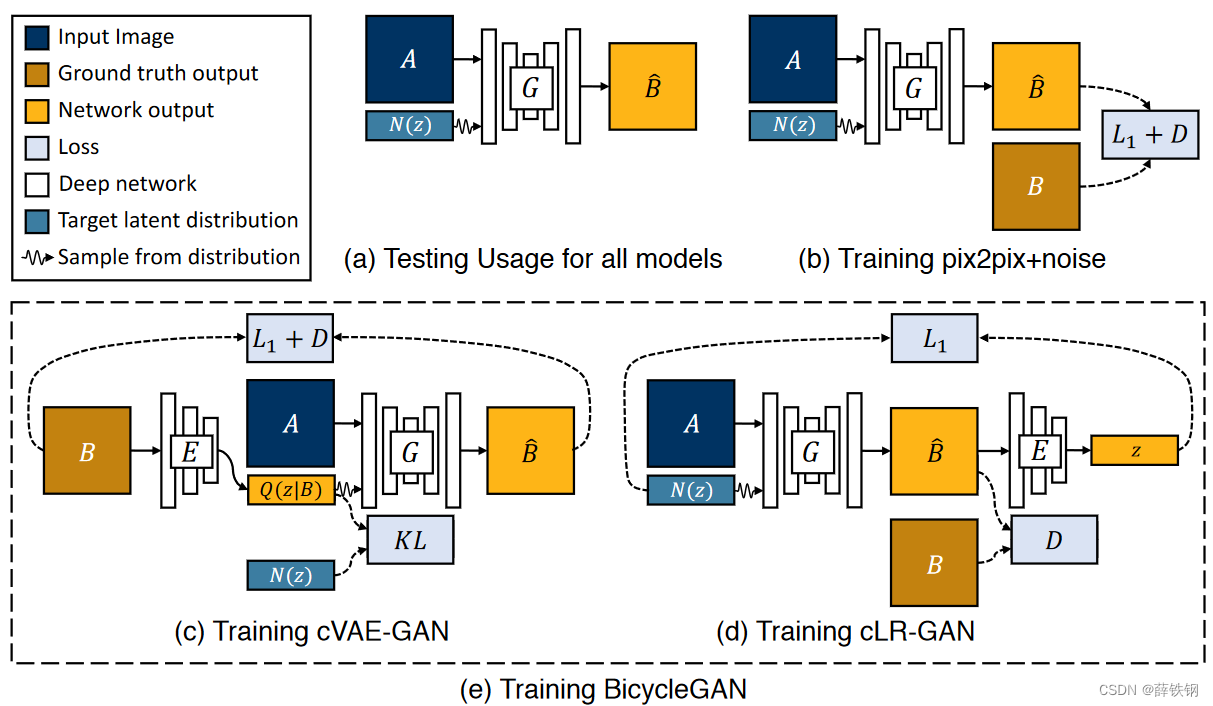
Figure 2: Overview: (a) Test time usage of all the methods. To produce a sample output, a latent code $z$ is first randomly sampled from a known distribution (e.g., a standard normal distribution). A generator $G$ maps an input image $\mathbf{A}$ (blue) and the latent sample $z$ to produce a output sample $\hat{\mathbf{B}}$ (yellow). (b) pix2pix+noise [20] baseline, with an additional ground truth image $\mathbf{B}$ (brown) that corresponds to $\mathbf{A}$. $(c)$ cVAE-GAN (and cAE-GAN) starts from a ground truth target image $\mathbf{B}$ and encode it into the latent space. The generator then attempts to map the input image $\mathbf{A}$ along with a sampled z back into the original image $\mathbf{B}$. (d) cLR-GAN randomly samples a latent code from a known distribution, uses it to map $\mathbf{A}$ into the output $\hat{\mathbf{B}}$, and then tries to reconstruct the latent code from the output. (e) Our hybrid BicycleGAN method combines constraints in both directions.

图 2：概览： (a) 所有方法的测试时间使用情况。要生成样本输出，首先要从已知分布（如标准正态分布）中随机抽取隐码 $z$。生成器 $G$ 映射输入图像 $\mathbf{A}$（蓝色）和潜在样本 $z$，生成输出样本 $\hat{\mathbf{B}}$（黄色）。$(c)$ cVAE-GAN（和 cAE-GAN）从ground-truth图像 $\mathbf{B}$ 开始，将其编码到隐空间。(d) cLR-GAN 从已知分布中随机采样隐码，用它将 $\mathbf{A}$ 映射到输出 $\hat{\mathbf{B}}$，然后尝试从输出中重建隐码。(e) 我们的混合 BicycleGAN 方法结合了两个方向的约束。

Our goal is to learn a multi-modal mapping between two image domains, for example, edges and photographs, or night and day images, etc. Consider the input domain $\mathcal{A}\subset {\mathbb{R}}^{H\times W\times 3}$, which is to be mapped to an output domain $\mathcal{B}\subset {\mathbb{R}}^{H\times W\times 3}$. During training, we are given a dataset of paired instances from these domains, { ( A ∈ A , B ∈ B ) } \left\{(\mathbf{A}{\in}\mathcal{A},\mathbf{B}{\in}\mathcal{B})\right\} {(A∈A,B∈B)}, which is representative of a joint distribution $p(\mathbf{A},\mathbf{B})$. It is important to note that there could be multiple plausible paired instances $\mathbf{B}$ that would correspond to an input instance $\mathbf{A}$, but the training dataset usually contains only one such pair. However, given a new instance $\mathbf{A}$ during test time, our model should be able to generate a diverse set of output $\hat{\mathbf{B}}$’s, corresponding to different modes in the distribution $p(B|A)$.

我们的目标是学习两个图像域之间的多模态映射，例如边缘草图和照片，或夜晚和白天的图像等。考虑输入域 $\mathcal{A}\subset {\mathbb{R}}^{H\times W\times 3}$ ，它将被映射到输出域 $\mathcal{B}\subset {\mathbb{R}}^{H\times W\times 3}$ 。在训练过程中，我们会得到来自这些域的配对实例数据集，即 { ( A ∈ A , B ∈ B ) } \left\{(\mathbf{A}{\in}\mathcal{A},\mathbf{B}{\in}\mathcal{B})\right\} {(A∈A,B∈B)}，该数据集代表了联合分布 $p(\mathbf{A},\mathbf{B})$。值得注意的是，可能有多个可信的配对实例 $\mathbf{B}$ 与输入实例 $\mathbf{A}$ 相对应，但训练数据集通常只包含一个这样的配对。然而，在测试期间给定一个新的实例 $\mathbf{A}$，我们的模型应该能够生成一组不同的输出 $\hat{\mathbf{B}}$，对应于分布 $p(B|A)$ 中的不同模式。

While conditional GANs have achieved success in image-to-image translation tasks [20, 34, 40, 45, 47, 55], they are primarily limited to generating a deterministic output $\hat{\mathbf{B}}$ given the input image $\mathbf{A}$. On the other hand, we would like to learn the mapping that could sample the output $\hat{\mathbf{B}}$ from true conditional distribution given $\mathbf{A}$, and produce results which are both diverse and realistic. To do so, we learn a low-dimensional latent space $\mathbf{z}\in {\mathbb{R}}^Z$, which encapsulates the ambiguous aspects of the output mode which are not present in the input image. For example, a sketch of a shoe could map to a variety of colors and textures, which could get compressed in this latent code. We then learn a deterministic mapping $G:(\mathbf{A},\mathbf{z})\to \mathbf{B}$ to the output. To enable stochastic sampling, we desire the latent code vector $z$ to be drawn from some prior distribution $p(\mathbf{z})$; we use a standard Gaussian distribution $\mathcal{N}(0,I)$ in this work.

虽然条件 GANs 在图像到图像的转换任务中取得了成功[20, 34, 40, 45, 47, 55]，但它们主要局限于在输入图像 $\mathbf{A}$ 的情况下生成确定性输出 $\hat{\mathbf{B}}$。另一方面，我们希望学习一种映射，这种映射可以从给定 $\mathbf{A}$ 的真实条件分布中对输出 $\hat{\mathbf{B}}$ 进行采样，并产生既多样又真实的结果。为此，我们学习了一个低维的潜在空间 $\mathbf{z}\in {\mathbb{R}}^Z$ ，它包含了输出模式中不存在于输入图像中的模糊方面。例如，一张鞋子的草图可以映射出多种颜色和纹理，这些都可以在这个隐代码中得到压缩。然后，我们就可以学习到输出的确定性映射 $G:(\mathbf{A},\mathbf{z})\to \mathbf{B}$。为了实现随机抽样，我们希望从某种先验分布 $p(\mathbf{z})$ 中抽取隐码向量 $z$；在这项工作中，我们使用了标准高斯分布 $\mathcal{N}(0,I)$。

We first discuss a simple extension of existing methods and discuss its strengths and weakness, motivating the development of our proposed approach in the subsequent subsections.

我们首先讨论现有方法的一个简单扩展，并讨论其优缺点，从而在随后的小节中提出我们所建议的方法。

3.1 Baseline: pix2pix+noise $(\mathbf{z}\to \hat{\mathbf{B}})$

The recently proposed pix2pix model [20] has shown high quality results in the image-to-image translation setting. It uses conditional adversarial networks [15, 30] to help produce perceptually realistic results. GANs train a generator $G$ and discriminator $D$ by formulating their objective as an adversarial game. The discriminator attempts to differentiate between real images from the dataset and fake samples produced by the generator. Randomly drawn noise z is added to attempt to induce stochasticity. We illustrate the formulation in Figure 2(b) and describe it below.
${\mathcal{L}}_{\mathrm{GAN}}(G,D)={\mathbb{E}}_{\mathbf{A},\mathbf{B}\sim p(\mathbf{A},\mathbf{B})}[\log (D(\mathbf{A},\mathbf{B}))]+{\mathbb{E}}_{\mathbf{A}\sim p(\mathbf{A}),\mathbf{z}\sim p(\mathbf{z})}[\log (1-D(\mathbf{A},G(\mathbf{A},\mathbf{z})))](1)$

最近提出的 pix2pix 模型[20]在图像到图像的转换设置中显示出高质量的结果。它使用条件对抗网络 [15, 30] 来帮助产生感知真实的结果。GANs 通过将其目标表述为对抗性博弈来训练生成器 $G$ 和判别器 $D$。判别器试图区分数据集中的真实图像和生成器生成的虚假样本。随机抽取的噪声 z 被添加进来，试图诱发随机性。我们在图 2(b) 中说明了这一公式，并在下文中加以描述。
${\mathcal{L}}_{\mathrm{GAN}}(G,D)={\mathbb{E}}_{\mathbf{A},\mathbf{B}\sim p(\mathbf{A},\mathbf{B})}[\log (D(\mathbf{A},\mathbf{B}))]+{\mathbb{E}}_{\mathbf{A}\sim p(\mathbf{A}),\mathbf{z}\sim p(\mathbf{z})}[\log (1-D(\mathbf{A},G(\mathbf{A},\mathbf{z})))](1)$

To encourage the output of the generator to match the input as well as stabilize the training, we use an ${\ell }_1$ loss between the output and the ground truth image.
${\mathcal{L}}_1^{\mathrm{image}}(G)={\mathbb{E}}_{\mathbf{A},\mathbf{B}\sim p(\mathbf{A},\mathbf{B}),\mathbf{z}\sim p(\mathbf{z})}||\mathcal{B}-G(\mathbf{A},\mathbf{z})|{|}_1(2)$

为了使生成器的输出与输入相匹配，并稳定训练结果，我们在输出和ground-truth图像之间使用了 ${\ell }_1$ 损失。
${\mathcal{L}}_1^{\mathrm{image}}(G)={\mathbb{E}}_{\mathbf{A},\mathbf{B}\sim p(\mathbf{A},\mathbf{B}),\mathbf{z}\sim p(\mathbf{z})}||\mathcal{B}-G(\mathbf{A},\mathbf{z})|{|}_1(2)$

The final loss function uses the GAN and ${\ell }_1$ terms, balanced by $\lambda$.
$G^{\ast }=\arg {\min }_G{\max }_D{\mathcal{L}}_{\mathrm{GAN}}(G,D)+\lambda {\mathcal{L}}_1^{\mathrm{image}}(G)(3)$

最终的损失函数使用 GAN 和 ${\ell }_1$ 项，并由 $\lambda$ 进行平衡。
$G^{\ast }=\arg {\min }_G{\max }_D{\mathcal{L}}_{\mathrm{GAN}}(G,D)+\lambda {\mathcal{L}}_1^{\mathrm{image}}(G)(3)$

In this scenario, there is little incentive for the generator to make use of the noise vector which encodes random information. Isola et al. [20] note that the noise was ignored by the generator in preliminary experiments and was removed from the final experiments. This was consistent with observations made in the conditional settings by [29, 34], as well as the mode collapse phenomenon observed in unconditional cases [14, 39]. In this paper, we explore different ways to explicitly enforce the latent coding to capture relevant information.

在这种情况下，生成器几乎没有动机利用编码随机信息的噪声向量。Isola等人[20]注意到，在初步实验中，噪声被发生器忽略，在最终实验中被去除。这与[29,34]在条件条件下的观察结果以及在无条件情况下观察到的模态坍缩现象[14,39]是一致的。在本文中，我们探索了不同的方法来显式地执行隐码以捕获相关信息。

3.2 Conditional Variational Autoencoder GAN: cVAE-GAN $(\mathbf{B}\to \mathbf{z}\to \hat{\mathbf{B}})$

One way to force the latent code $z$ to be “useful" is to directly map the ground truth $\mathbf{B}$ to it using an encoding function $E$. The generator $G$ then uses both the latent code and the input image $\mathbf{A}$ to synthesize the desired output $\hat{\mathbf{B}}$. The overall model can be easily understood as the reconstruction of $\mathbf{B}$, with latent encoding $z$ concatenated with the paired $A$ in the middle – similar to an autoencoder [18]. This interpretation is better shown in Figure 2$(c)$.

迫使隐码 $z$ 变得 "有用 "的一种方法是使用编码函数 $E$ 将ground-truth $\mathbf{B}$ 直接映射到隐码 $z$ 上。然后，生成器 $G$ 使用隐码和输入图像 $\mathbf{A}$ 合成所需的输出 $\hat{\mathbf{B}}$。整个模型可以很容易地理解为重建 $\mathbf{B}$，中间用隐码 $z$ 与配对的 $A$ 连接–类似于自动编码器 [18]。图 2$(c)$更好地诠释了这一点。

This approach has been successfully investigated in Variational Autoencoder [23] in the unconditional scenario without the adversarial objective. Extending it to conditional scenario, the distribution $Q(z|B)$ of latent code $z$ using the encoder $E$ with a Gaussian assumption, $Q(\mathbf{z}|\mathbf{B})\triangleq E(\mathbf{B})$. To reflect this, Equation 1 is modified to sampling $\mathbf{z}\sim E(\mathbf{B})$ using the re-parameterization trick, allowing direct back-propagation [23].
${\mathcal{L}}_{\mathrm{GAN}}^{\mathrm{VAE}}={\mathbb{E}}_{\mathbf{A},\mathbf{B}\sim p(\mathbf{A},\mathbf{B})}[\log (D(\mathbf{A},\mathbf{B}))]+{\mathbb{E}}_{\mathbf{A},\mathbf{B}\sim p(\mathbf{A},\mathbf{B}),\mathbf{z}\sim E(\mathbf{B})}[\log (1-D(\mathbf{A},G(\mathbf{A},\mathbf{z})))](4)$

在无对抗目标的无条件情况下，变异自动编码器 [23] 成功研究了这种方法。将其扩展到有条件情况下，使用高斯假设的编码器 $E$ 时，隐码 $z$ 的分布 $Q(\mathbf{z}|\mathbf{B})\triangleq E(\mathbf{B})$ 为高斯假设，$Q(\mathbf{z}|\mathbf{B})\triangleq E(\mathbf{B})$。为了反映这一点，等式 1 被修改为使用重参数化技巧对 $\mathbf{z}\sim E(\mathbf{B})$ 进行采样，从而允许直接反向传播 [23]。
${\mathcal{L}}_{\mathrm{GAN}}^{\mathrm{VAE}}={\mathbb{E}}_{\mathbf{A},\mathbf{B}\sim p(\mathbf{A},\mathbf{B})}[\log (D(\mathbf{A},\mathbf{B}))]+{\mathbb{E}}_{\mathbf{A},\mathbf{B}\sim p(\mathbf{A},\mathbf{B}),\mathbf{z}\sim E(\mathbf{B})}[\log (1-D(\mathbf{A},G(\mathbf{A},\mathbf{z})))](4)$

We make the corresponding change in the ${\ell }_1$ loss term in Equation 2 as well to obtain ${\mathcal{L}}_1^{\mathrm{VAE}}(G)={\mathbb{E}}_{\mathbf{A},\mathbf{B}\sim p(\mathbf{A},\mathbf{B}),\mathbf{z}\sim E(\mathbf{B})}||\mathbf{B}-G(\mathbf{A},\mathbf{z})|{|}_1$. Further, the latent distribution encoded by $E(B)$ is encouraged to be close to a random Gaussian to enable sampling at inference time, when $\mathbf{B}$ is not known.
${\mathcal{L}}_{\mathrm{KL}}(E)={\mathbb{E}}_{\mathbf{B}\sim p(\mathbf{B})}[{\mathcal{D}}_{\mathrm{KL}}(E(\mathbf{B})||\mathcal{N}(0,I))],(5)$

我们对等式 2 中的 ${\ell }_1$ 损失项也做了相应的改变，得到 ${\mathcal{L}}_1^{\mathrm{VAE}}(G)={\mathbb{E}}_{\mathbf{A}、\mathbf{B}\sim p(\mathbf{A},\mathbf{B}),\mathbf{z}\sim E(\mathbf{B})}||\mathbf{B}-G(\mathbf{A},\mathbf{z})|{|}_1$. 此外，当 $\mathbf{B}$ 未知时，鼓励由 $E(B)$ 编码的潜在分布接近随机高斯分布，以便在推理时进行采样。
${\mathcal{L}}_{\mathrm{KL}}(E)={\mathbb{E}}_{\mathbf{B}\sim p(\mathbf{B})}[{\mathcal{D}}_{\mathrm{KL}}(E(\mathbf{B})||\mathcal{N}(0,I))],(5)$

where ${\mathcal{D}}_{\mathrm{KL}}(p||q)=-\int p(z)\log \frac{p(z)}{q(z)}dz$.This forms our cVAE-GAN objective, a conditional version of the VAE-GAN [26] as
$G^{\ast },E^{\ast }=\arg {\min }_{G,E}{\max }_D{\mathcal{L}}_{\mathrm{GAN}}^{\mathrm{VAE}}(G,D,E)+\lambda {\mathcal{L}}_1^{\mathrm{VAE}}(G,E)+{\lambda }_{\mathrm{KL}}{\mathcal{L}}_{\mathrm{KL}}(E).(6)$

其中${\mathcal{D}}_{\mathrm{KL}}(p||q)=-\int p(z)\log \frac{p(z)}{q(z)}dz$，这就形成了我们的cVAE-GAN目标，即VAE-GAN[26]的条件版本
$G^{\ast },E^{\ast }=\arg {\min }_{G,E}{\max }_D{\mathcal{L}}_{\mathrm{GAN}}^{\mathrm{VAE}}(G,D,E)+\lambda {\mathcal{L}}_1^{\mathrm{VAE}}(G,E)+{\lambda }_{\mathrm{KL}}{\mathcal{L}}_{\mathrm{KL}}(E).(6)$

As a baseline, we also consider the deterministic version of this approach, i.e., dropping KLdivergence and encoding $\mathbf{z}=E(\mathbf{B})$. We call it cAE-GAN and show a comparison in the experiments. There is no guarantee in cAE-GAN on the distribution of the latent space $\mathbf{z}$, which makes the test-time sampling of $\mathbf{z}$ difficult.

作为基准，我们还考虑了这种方法的确定性版本，即去掉KLdivergence并编码$\mathbf{z}=E(\mathbf{B})$。我们称之为cAE-GAN，并在实验中进行了比较。在cAE-GAN中，对于潜在空间$\mathbf{z}$的分布没有保证，这使得$\mathbf{z}$的测试时间采样变得困难。

3.3 Conditional Latent Regressor GAN: cLR-GAN$(\mathbf{z}\to \hat{\mathbf{B}}\to \hat{\mathbf{z}})$

We explore another method of enforcing the generator network to utilize the latent code embedding $\mathbf{z}$, while staying close to the actual test time distribution $p(\mathbf{z})$, but from the latent code’s perspective. As shown in Figure 2(d), we start from a randomly drawn latent code $\mathbf{z}$ and attempt to recover it with $\hat{\mathbf{z}}=E(G(\mathbf{A},\mathbf{z}))$. Note that the encoder $E$ here is producing a point estimate for $\hat{\mathbf{z}}$, whereas the encoder in the previous section was predicting a Gaussian distribution.
${\mathcal{L}}_1^{\mathrm{latent}}(G,E)={\mathbb{E}}_{\mathbf{A}\sim p(\mathbf{A}),\mathbf{z}\sim p(\mathbf{z})}||\mathbf{z}-E(G(\mathbf{A},\mathbf{z}))|{|}_1(7)$

我们探索了另一种方法来强制生成器网络利用嵌入$\mathbf{z}$的潜在代码，同时保持接近实际测试时间分布$p(\mathbf{z})$，但从潜在代码的角度来看。如图2(d)所示，我们从随机绘制的潜在代码$\mathbf{z}$开始，并尝试使用$\hat{\mathbf{z}}=E(G(\mathbf{a}，\mathbf{z}))$来恢复它。注意，这里的编码器$E$生成$\hat{\mathbf{z}}$的点估计，而上一节中的编码器预测的是高斯分布。
${\mathcal{L}}_1^{\mathrm{latent}}(G,E)={\mathbb{E}}_{\mathbf{A}\sim p(\mathbf{A}),\mathbf{z}\sim p(\mathbf{z})}||\mathbf{z}-E(G(\mathbf{A},\mathbf{z}))|{|}_1(7)$

We also include the discriminator loss $L_{\mathrm{GAN}}(G,D)$ (Equation 1) on $\hat{\mathbf{B}}$, to encourage the network to generate realistic results, and the full loss can be written as:
$G^{\ast },E^{\ast }=\arg {\min }_{G,E}{\max }_D{\mathcal{L}}_{\mathrm{GAN}}(G,D)+{\lambda }_{\mathrm{latent}}{\mathcal{L}}_1^{\mathrm{latent}}(G,E)(8)$

我们还在$\hat{\mathbf{B}}$上加入了判别器损失$L_{mathbfGAN}(G,D)$(方程1)，以鼓励网络产生真实的结果，其完全损失可以表示为:
$G^{\ast },E^{\ast }=\arg {\min }_{G,E}{\max }_D{\mathcal{L}}_{\mathrm{GAN}}(G,D)+{\lambda }_{\mathrm{latent}}{\mathcal{L}}_1^{\mathrm{latent}}(G,E)(8)$

The ${\ell }_1$ loss for the ground truth image $\mathbf{B}$ is not used. Since the noise vector is randomly drawn, the predicted $\hat{\mathbf{B}}$ does not necessarily need to be close to the ground truth but does need to be realistic. The above objective bears similarity to the “latent regressor" model [4, 8, 10], where the generated sample $\hat{\mathbf{B}}$ is encoded to generate a latent vector.

没有使用ground-truth图像$\mathbf{B}$的${\ell }_1$损失。由于噪声向量是随机绘制的，因此预测的$\hat{\mathbf{B}}$不一定需要接近基本事实，但需要是现实的。上述目标与“潜在回归”模型[4,8,10]相似，其中生成的样本$\hat{\mathbf{B}}$被编码以生成潜在向量。

3.4 Our Hybrid Model: BicycleGAN

We combine the cVAE-GAN and cLR-GAN objectives in a hybrid model. For cVAE-GAN, the encoding is learned from real data, but a random latent code may not yield realistic images at test time – the KL loss may not be well optimized. Perhaps more importantly, the adversarial classifier D does not have a chance to see results sampled from the prior during training. In cLR-GAN, the latent space is easily sampled from a simple distribution, but the generator is trained without the benefit of seeing ground truth input-output pairs. We propose to train with constraints in both directions, aiming to take advantage of both cycles $(\mathrm{B}\to \mathrm{z}\to \hat{\mathrm{B}}\mathrm{and}\mathrm{z}\to \hat{\mathrm{B}}\to \hat{\mathrm{z}})$, hence the name BicycleGAN.
$\begin{array}{rlr}{G}^{\ast },E^{\ast }=\arg \underset{G,E}{\min }\underset{D}{\max }& {\mathcal{L}}_{\mathrm{GAN}}^{\mathrm{VAE}}(G,D,E)+\lambda {\mathcal{L}}_1^{\mathrm{VAE}}(G,E)& \\ & & \text{(9)}\\ & +{\mathcal{L}}_{\mathrm{GAN}}(G,D)+{\lambda }_{\mathrm{latent}}{\mathcal{L}}_1^{\mathrm{latent}}(G,E)+{\lambda }_{\mathrm{KL}}{\mathcal{L}}_{\mathrm{KL}}(E),& \end{array}$
where the hyper-parameters $lambda$, $lambd{a}_{latent}$, and $lambd{a}_{KL}$control the relative importance of each term.

我们将cVAE-GAN和cLR-GAN目标结合在一个混合模型中。对于cVAE-GAN，编码是从真实数据中学习的，但是随机潜在代码在测试时可能无法产生真实的图像- KL损失可能没有得到很好的优化。也许更重要的是，在训练期间，对抗性分类器D没有机会看到从先前的分类器中采样的结果。在cLR-GAN中，潜在空间很容易从一个简单的分布中采样，但是生成器的训练没有看到地面真值输入输出对的好处。我们建议在两个方向上进行约束训练，目的是利用这两个周期
$\begin{array}{rlr}{G}^{\ast },E^{\ast }=\arg \underset{G,E}{\min }\underset{D}{\max }& {\mathcal{L}}_{\mathrm{GAN}}^{\mathrm{VAE}}(G,D,E)+\lambda {\mathcal{L}}_1^{\mathrm{VAE}}(G,E)& \\ & & \text{(9)}\\ & +{\mathcal{L}}_{\mathrm{GAN}}(G,D)+{\lambda }_{\mathrm{latent}}{\mathcal{L}}_1^{\mathrm{latent}}(G,E)+{\lambda }_{\mathrm{KL}}{\mathcal{L}}_{\mathrm{KL}}(E),& \end{array}$
其中超参数$lambda$， $lambd{a}_{latent}$和$lambd{a}_{KL}$控制每个项的相对重要性。

In the unconditional GAN setting, Larsen et al. [26] observe that using samples from both the prior $\mathcal{N}(0,I)$ and encoded $E(\mathbf{B})$ distributions further improves results. Hence, we also report one variant which is the full objective shown above (Equation 9), but without the reconstruction loss on the latent space ${\mathcal{L}}_1^{\mathrm{latent}}$. We call it cVAE-GAN++, as it is based on cVAE-GAN with an additional loss ${\mathcal{L}}_{\mathrm{GAN}}(G,D)$, which allows the discriminator to see randomly drawn samples from the prior.

在无条件GAN设置中，Larsen等人[26]观察到，使用来自先验$\mathcal{N}(0,I)$和编码器$E(\mathbf{B})$分布的样本进一步改善了结果。因此，我们也报告了一个变体，它是上面所示的完整目标(公式9)，但没有在潜在空间${\mathcal{L}}_1^{\mathrm{latent}}$上的重建损失。我们称之为cVAE-GAN++，因为它是基于cVAE-GAN加上一个额外的损失${\mathcal{L}}_{\mathrm{GAN}}(G,D)$，这使得鉴别器可以看到从先验中随机抽取的样本。

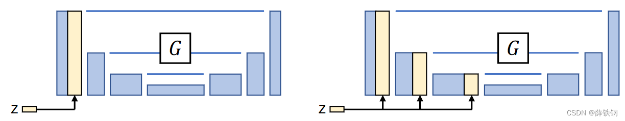
Figure 3: Alternatives for injecting $z$ into generator. Latent code $z$ is injected by spatial replication and concatenation into the generator network. We tried two alternatives, (left) injecting into the input layer and (right) every intermediate layer in the encoder.

图3：向生成器注入$z$的备选方案。隐码$z$通过空间复制和连接注入到生成器网络中。我们尝试了两种选择，(左)向输入层注入，(右)向编码器中的每个中间层注入。

4 Implementation Details

The code and additional results are publicly available at https://github.com/junyanz/ BicycleGAN. Please refer to our website for more details about the datasets, architectures, and training procedures.

代码和其他结果可在https://github.com/junyanz/ BicycleGAN上公开获得。请参考我们的网站了解更多关于数据集、架构和训练程序的详细信息。

Network architecture For generator $G$, we use the U-Net [37], which contains an encoder-decoder architecture, with symmetric skip connections. The architecture has been shown to produce strong results in the unimodal image prediction setting when there is a spatial correspondence between input and output pairs. For discriminator $D$, we use two PatchGAN discriminators [20] at different scales, which aims to predict real vs. fake for 70 × 70 and 140 × 140 overlapping image patches. For the encoder $E$, we experiment with two networks: (1) $E_{CNN}$: CNN with a few convolutional and downsampling layers and (2) $E_{ResNet}$: a classifier with several residual blocks [17].

网络结构 对于生成器$G$，我们使用U-Net[37]，它包含一个具有对称跳过连接的编码器-解码器架构。当输入和输出对之间存在空间对应时，该架构已被证明在单峰图像预测设置中产生强大的结果。对于判别器$D$，我们使用了两个不同尺度的PatchGAN判别器[20]，旨在预测70 × 70和140 × 140重叠图像patch的真假。对于编码器$E$，我们使用两个网络进行实验:(1)$E_{CNN}$:具有几个卷积和下采样层的CNN， (2) $E_{ResNet}$:具有多个残差块的分类器[17]。

Training details We build our model on the Least Squares GANs (LSGANs) variant [28], which uses a least-squares objective instead of a cross entropy loss. LSGANs produce high-quality results with stable training. We also find that not conditioning the discriminator $D$ on input $A$ leads to better results (also discussed in [34]), and hence choose to do the same for all methods. We set the parameters ${\lambda }_{image}=10$, ${\lambda }_{latent}=0.5$ and ${\lambda }_{KL}=0.01$ in all our experiments. We tie the weights for the generators and encoders in the cVAE-GAN and cLR-GAN models. For the encoder, only the predicted mean is used in cLR-GAN. We observe that using two separate discriminators yields slightly better visual results compared to sharing weights. We only update G for the ${\ell }_1$ loss ${\mathcal{L}}_1^{\mathrm{latent}}(G,E)$ on the latent code (Equation 7), while keeping E fixed. We found optimizing G and E simultaneously for the loss would encourage G and E to hide the information of the latent code without learning meaningful modes. We train our networks from scratch using Adam [22] with a batch size of 1 and with a learning rate of 0.0002. We choose latent dimension $|\mathbf{z}|=8$ across all the datasets.

训练细节 我们的模型基于最小二乘 GANs（LSGANs）变体 [28]，它使用最小二乘目标而不是交叉熵损失。LSGANs 可以通过稳定的训练产生高质量的结果。我们还发现，不对输入 $A$ 的判别器 $D$ 进行条件化处理会带来更好的结果（这在 [34] 中也有讨论），因此我们选择对所有方法都采用同样的方法。我们在所有实验中都设置了参数${\lambda }_{image}=10$，${\lambda }_{latent}=0.5$，${\lambda }_{KL}=0.01$。在 cVAE-GAN 和 cLR-GAN 模型中，我们对生成器和编码器的权重进行了绑定。在 cLR-GAN 模型中，编码器只使用预测平均值。我们发现，与共享权重相比，使用两个独立的判别器会产生更好的视觉效果。我们只针对潜码上的 ${\ell }_1$ 损失 ${\mathcal{L}}_1^{\mathrm{latent}}(G,E)$ 更新 $G$（等式 7），而 $E$ 保持不变。我们发现，同时优化 $G$ 和 $E$ 的损失会促使 $G$ 和 $E$ 隐藏隐码信息，而无法学习到有意义的模式。我们使用 Adam [22]从头开始训练我们的网络，批量大小为 1，学习率为 0.0002。在所有数据集中，我们都选择了潜在维度 $|\mathbf{z}|=8$。

Injecting the latent code $\mathbf{z}$ to generator. We explore two ways of propagating the latent code z to the output, as shown in Figure 3: (1) add_to_input: we spatially replicate a Z-dimensional latent code z to an $H\times W\times Z$ tensor and concatenate it with the $H\times W\times 3$ input image and (2) add_to_all: we add $mathbfz$ to each intermediate layer of the network $G$, after spatial replication to the appropriate sizes.

向生成器注入隐码 $\mathbf{z}$ 我们探索了两种将潜码 $\mathbf{z}$传播到输出的方法，如图 3 所示：（1）add_to_input：我们将 Z 维潜码$\mathbf{z}$空间复制到一个 $H\times W\times Z$ 张量中，并将其与 $H\times W\times 3$ 输入图像连接起来；（2）add_to_all：我们将 $\mathbf{z}$ 添加到网络 $G$ 的每个中间层，然后将其空间复制到适当大小。

5 Experiments

Datasets We test our method on several image-to-image translation problems from prior work, including edges → photos [48, 54], Google maps → satellite [20], labels → images [5], and outdoor night → day images [25]. These problems are all one-to-many mappings. We train all the models on 256 × 256 images.

数据集 我们在之前工作的几个图像到图像的转换问题上测试了我们的方法，包括边缘→照片[48,54]，谷歌地图→卫星[20]，标签→图像[5]，以及户外夜间→白天图像[25]。这些问题都是一对多映射。我们在256 × 256的图像上训练所有的模型。

Methods We evaluate the following models described in Section 3: pix2pix+noise, cAE-GAN, cVAE-GAN, cVAE-GAN++, cLR-GAN, and our hybrid model BicycleGAN.

方法 我们评估了第3节中描述的以下模型:pix2pix+noise、cAE-GAN、cVAE-GAN、cVAE-GAN++、cLR-GAN和我们的混合模型BicycleGAN。

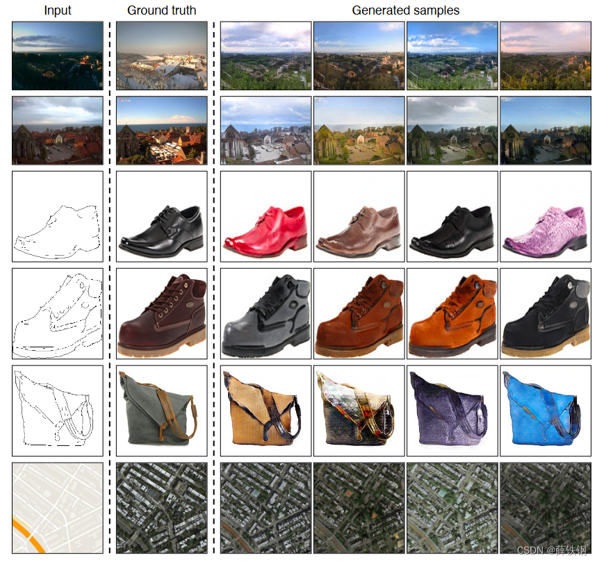
Figure 4: Example Results We show example results of our hybrid model BicycleGAN. The left column shows the input. The second shows the ground truth output. The final four columns show randomly generated samples. We show results of our method on night→day, edges→shoes, edges→handbags, and maps→satellites. Models and additional examples are available at https://junyanz.github.io/BicycleGAN.

图4：结果示例 我们展示了我们的混合模型BicycleGAN的示例结果。左列显示输入。第二列显示了ground-truth。最后四列显示随机生成的样本。我们展示了我们的方法在夜晚→白天、边缘→鞋子、边缘→手袋和地图→卫星上的结果。模型和其他示例可在https://junyanz.github.io/BicycleGAN上获得。

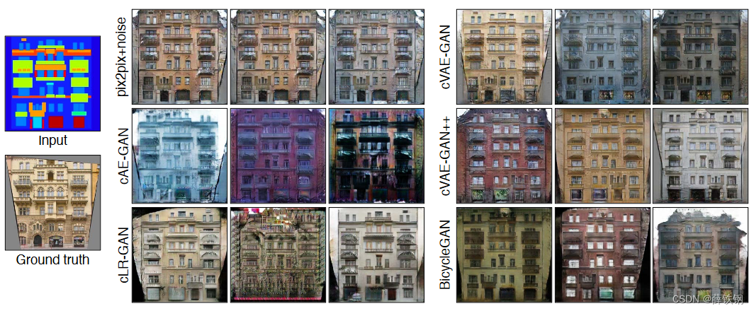
Figure 5: Qualitative method comparison We compare results on the labels → facades dataset across different methods. The BicycleGAN method produces results which are both realistic and diverse.

图5：定性方法比较 我们比较了不同方法在标签→facades数据集上的结果。BicycleGAN方法产生的结果既真实又多样。

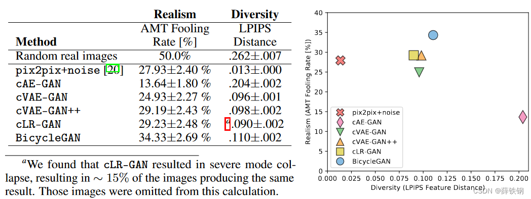
Figure 6: Realism vs Diversity We measure diversity using average LPIPS distance [52], and realism using a real vs. fake Amazon Mechanical Turk test on the Google maps → satellites task. The pix2pix+noise baseline produces little diversity. Using only cAE-GAN method produces large artifacts during sampling. The hybrid BicycleGAN method, which combines cVAE-GAN and cLR-GAN, produces results which have higher realism while maintaining diversity.

图6：现实性vs多样性 我们使用平均LPIPS距离来衡量多样性[52]，并在Google maps→卫星任务上使用真实与虚假的Amazon Mechanical Turk测试来衡量真实感。pix2pix+噪声基线产生的多样性很小。仅使用cAE-GAN方法会在采样过程中产生较大的伪影。结合cVAE-GAN和cLR-GAN的混合BicycleGAN方法，在保持多样性的同时，获得了更高的真实感。

5.1 Qualitative Evaluation

We show qualitative comparison results on Figure 5. We observe that pix2pix+noise typically produces a single realistic output, but does not produce any meaningful variation. cAE-GAN adds variation to the output, but typically at a large cost to result quality. An example on facades is shown on Figure 4.

我们在图5中显示了定性比较结果。我们观察到，pix2pix+noise 通常会产生一个真实的输出，但不会产生任何有意义的变化。cAE-GAN增加了输出的变化，但通常以结果质量为代价。图4显示了一个关于facade的示例。

We observe more variation in the cVAE-GAN, as the latent space is encouraged to encode information about ground truth outputs. However, the space is not densely populated, so drawing random samples may cause artifacts in the output. The cLR-GAN shows less variation in the output, and sometimes suffers from mode collapse. When combining these methods, however, in the hybrid method BicycleGAN, we observe results which are both diverse and realistic. Please see our website for a full set of results.

我们在cVAE-GAN中观察到更多的变化，因为潜在空间被鼓励编码有关ground-truth输出的信息。然而，空间不是密集的，因此绘制随机样本可能会导致输出中的伪影。cLR-GAN的输出变化较小，有时会出现模式崩溃。然而，当结合这些方法时，在混合方法BicycleGAN中，我们观察到的结果既多样又现实。请访问我们的网站查看完整的结果。

5.2 Quantitative Evaluation

We perform a quantitative analysis of the diversity, realism, and latent space distribution on our six variants and baselines. We quantitatively test the Google maps → satellites dataset.

我们对六个变体和基线的多样性、真实性和潜空间分布进行了定量分析。我们对谷歌地图 → 卫星数据集进行了定量测试。

Diversity We compute the average distance of random samples in deep feature space. Pretrained networks have been used as a “perceptual loss" in image generation applications [9, 12, 21], as well as a held-out “validation" score in generative modeling, for example, assessing the semantic quality and diversity of a generative model [39] or the semantic accuracy of a grayscale colorization [50].

多样性 我们计算深度特征空间中随机样本的平均距离。预训练网络已被用作图像生成应用中的 “感知损失”[9, 12, 21]，以及生成模型中的 "验证 "得分，例如，评估生成模型的语义质量和多样性[39]或灰度着色的语义准确性[50]。

In Figure 6, we show the diversity-score using the LPIPS metric proposed by [52]. For each method, we compute the average distance between 1900 pairs of randomly generated output $\hat{\mathbf{B}}$ images (sampled from 100 input $\mathbf{A}$ images). Random pairs of ground truth real images in the $\mathbf{B}\in \mathcal{B}$ domain produce an average variation of .262. As we are measuring samples $\hat{\mathbf{B}}$ which correspond to a specific input $\mathbf{A}$, a system which stays faithful to the input should definitely not exceed this score.

在图 6 中，我们展示了使用 [52] 提出的 LPIPS 指标得出的多样性分数。对于每种方法，我们都计算了 1900 对随机生成的输出 $\hat{\mathbf{B}}$ 图像（从 100 张输入 $\mathbf{A}$ 图像中采样）之间的平均距离。在$\mathbf{B}\in \mathcal{B}$域中，随机生成的一对地面真实图像的平均距离为 0.262。由于我们测量的是与特定输入 $\mathbf{A}$ 相对应的 $hat\mathbf{B}$ 样本，因此一个忠实于输入的系统绝对不会超过这个分数。

The pix2pix system [20] produces a single point estimate. Adding noise to the system pix2pix+noise produces a small diversity score, confirming the finding in [20] that adding noise does not produce large variation. Using the cAE-GAN model to encode a ground truth image B into a latent code z does increase the variation. The cVAE-GAN, cVAE-GAN++, and BicycleGAN models all place explicit constraints on the latent space, and the cLR-GAN model places an implicit constraint through sampling. These four methods all produce similar diversity scores. We note that high diversity scores may also indicate that unnatural images are being generated, causing meaningless variations. Next, we investigate the visual realism of our samples.

pix2pix 系统[20]产生的是单点估计值。在 pix2pix+noise 系统中加入噪声后，多样性得分很小，这证实了文献[20]中的结论，即加入噪声不会产生大的变化。使用 cAE-GAN 模型将地面真实图像 B 编码成潜在代码 z 确实会增加变化。cVAE-GAN、cVAE-GAN++ 和 BicycleGAN 模型都对潜空间施加了显式约束，而 cLR-GAN 模型则通过采样施加了隐式约束。这四种方法都能产生相似的多样性得分。我们注意到，高多样性得分也可能表明生成的图像不自然，造成了无意义的变化。接下来，我们将研究样本的视觉真实性。

Perceptual Realism To judge the visual realism of our results, we use human judgments, as proposed in [50] and later used in [20, 55]. The test sequentially presents a real and generated image to a human for 1 second each, in a random order, asks them to identify the fake, and measures the “fooling" rate. Figure 6(left) shows the realism across methods. The pix2pix+noise model achieves high realism score, but without large diversity, as discussed in the previous section. The cAE-GAN helps produce diversity, but this comes at a large cost to the visual realism. Because the distribution of the learned latent space is unclear, random samples may be from unpopulated regions of the space. Adding the KL-divergence loss in the latent space, used in the cVAE-GAN model, recovers the visual realism. Furthermore, as expected, checking randomly drawn z vectors in the cVAE-GAN++ model slightly increases realism. The cLR-GAN, which draws z vectors from the predefined distribution randomly, produces similar realism and diversity scores. However, the cLR-GAN model resulted in large mode collapse - approximately 15% of the outputs produced the same result, independent of the input image. The full hybrid BicycleGAN gets the best of both worlds, as it does not suffer from mode collapse and also has the highest realism score by a significant margin.

感知现实主义 为了判断结果的视觉逼真度，我们采用了人类判断的方法，这种方法在 [50] 中提出，后来在 [20, 55] 中使用。测试以随机顺序向人类展示真实图像和生成图像各 1 秒钟，要求他们识别假图像，并测量 "愚弄 "率。图 6（左）显示了各种方法的逼真度。pix2pix+noise 模型获得了较高的逼真度分数，但没有较大的多样性，这一点在上一节已经讨论过。cAE-GAN 有助于产生多样性，但这是以视觉逼真度为代价的。因为所学潜空间的分布并不明确，随机样本可能来自空间中没有填充的区域。在潜空间中添加 cVAE-GAN 模型中使用的 KL-发散损失，可以恢复视觉真实感。此外，正如预期的那样，在 cVAE-GAN++ 模型中检查随机绘制的 z 向量会略微增加真实感。从预定义分布中随机抽取 z 向量的 cLR-GAN 产生了相似的逼真度和多样性得分。不过，cLR-GAN 模型导致了较大的模式崩溃–大约 15%的输出产生了相同的结果，与输入图像无关。完全混合的 BicycleGAN 可谓两全其美，不仅不会出现模式坍塌，而且逼真度得分也是最高的。

Encoder architecture In pix2pix, Isola et al. [20] conduct extensive ablation studies on discriminators and generators. Here we focus on the performance of two encoder architectures, $E_{CNN}$ and $E_{ResNet}$, for our applications on the maps and facades datasets. We find that $E_{ResNet}$ better encodes the output image, regarding the image reconstruction loss $||\mathbf{B}-G(\mathbf{A},E(B))|{|}_1$ on validation datasets as shown in Table 1. We use $E_{ResNet}$ in our final model.

编码器结构 在pix2pix中，Isola等[20]对鉴别器和发生器进行了广泛的消融研究。在这里，我们关注两种编码器架构的性能，$E_{CNN}$和$E_{ResNet}$，用于我们在地图和立面数据集上的应用程序。我们发现$E_{ResNet}$更好地编码输出图像，对于验证数据集上的图像重建损失$||\mathbf{B}-G(\mathbf{A}，E(B))|{|}_1$，如表1所示。我们在最终模型中使用$E_{ResNet}$。

Methods of injecting latent code We evaluate two ways of injecting latent code $\mathbf{z}$: add_to_input and add_to_all (Section 4), regarding the same reconstruction loss $||\mathbf{B}-G(\mathbf{A},E(B))|{|}_1$. Table 1 shows that two methods give similar performance. This indicates that the U_Net [37] can already propagate the information well to the output without the additional skip connections from $\mathbf{z}$. We use add_to_all method to inject noise in our final model.

注入隐码的方式 我们评估了两种注入隐码 $\mathbf{z}$ 的方法：add_to_input 和 add_to_all（第 4 节），关于相同的重构损失 $||\mathbf{B}-G(\mathbf{A},E(B))|{|}_1$。表 1 显示，两种方法的性能相似。这表明 U_Net [37] 已经可以很好地将信息传播到输出，而不需要 $\mathbf{z}$ 的额外跳转连接。我们使用 add_too_all 方法在最终模型中注入噪声。

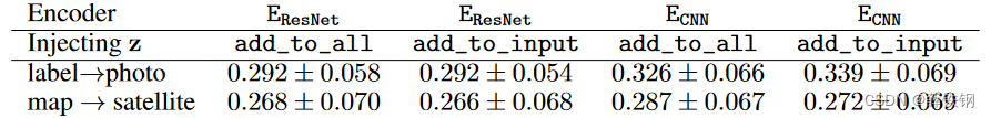
Table 1: The encoding performance with respect to the different encoder architectures and methods of injecting z. Here we report the reconstruction loss $||\mathbf{B}-G(\mathbf{A},E(B))|{|}_1$

表 1：不同编码器架构和注入 z 的方法的编码性能。在此，我们报告重建损失 $||\mathbf{B}-G(\mathbf{A},E(B))|{|}_1$

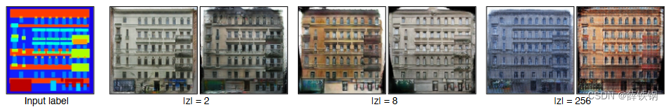
Figure 7: Different label → facades results trained with varying length of the latent code $\left|\mathrm{z}\right|\in 2,8,256$

图 7：用不同长度的隐码训练出的不同标签 → facades 结果$\left|\mathrm{z}\right|\in 2,8,256$

Latent code length We study the BicycleGAN model results with respect to the varying number of dimensions of latent codes {2, 8, 256} in Figure 7. A very low-dimensional latent code may limit the amount of diversity that can be expressed. On the contrary, a very high-dimensional latent code can potentially encode more information about an output image, at the cost of making sampling difficult. The optimal length of $\mathbf{z}$ largely depends on individual datasets and applications, and how much ambiguity there is in the output.

隐码长度 我们在图7中研究了关于隐码{2,8,256}的不同维数的BicycleGAN模型结果。一个非常低维的隐代码可能会限制可以表达的多样性的数量。相反，一个非常高维的隐码可以潜在地编码更多关于输出图像的信息，代价是采样变得困难。$\mathbf{z}$的最佳长度在很大程度上取决于不同的数据集和应用，以及输出结果的模糊程度。

6 Conclusions

In conclusion, we have evaluated a few methods for combating the problem of mode collapse in the conditional image generation setting. We find that by combining multiple objectives for encouraging a bijective mapping between the latent and output spaces, we obtain results which are more realistic and diverse. We see many interesting avenues of future work, including directly enforcing a distribution in the latent space that encodes semantically meaningful attributes to allow for image-to-image transformations with user controllable parameters.

总之，我们已经评估了一些在条件图像生成设置中对抗模式崩溃问题的方法。我们发现，通过结合多个目标来鼓励潜在空间和输出空间之间的双向映射，我们获得的结果更加真实和多样化。我们看到了许多有趣的未来工作途径，包括直接在潜在空间中强制执行一个分布，该分布对语义上有意义的属性进行编码，以允许使用用户可控参数进行图像到图像的转换。