


xodr文件(OpenDrive车道)解析原理并使用matplotlib进行二维可视化
目录
本文是关于opendrive道路格式文件xodr文件的解析和可视化的详细解析,以供有关研究者使用。xodr文件包含了车道的仿真地图,有时候我们需要针对性的进行开发,例如明确的知道每个车道的路沿绝对坐标等等。为了简化表示,本文采用二维可视化的任务将xodr文件进行解析和绘制。
因为篇幅限制,本文展示了部分关键脚本,建议读者参考本项目完整代码以了解详细的数据格式和技术细节,本项目的代码已经上传Github,供读者查阅:https://github.com/skx6/parse-and-visualize-xodr/tree/main,其中已经包含解析工具包,可以无障碍使用。
1. 基础知识
1.1 关于xodr文件
xodr文件是指OpenDRIVE(Open Drive)格式的道路数据文件。这种文件通常用于描述道路网络的拓扑结构、几何形状和其他相关属性,以便在仿真软件或自动驾驶系统中使用。
OpenDRIVE文件(.xodr)遵循XML(可扩展标记语言)格式,它由一系列标签和属性组成,用于描述道路网络的各个方面。以下是OpenDRIVE文件的基本结构和一些主要元素:
- 文件头部(Header):包含文件版本信息和一些基本的元数据,如制造商、创建日期等。
- 道路(Roads):描述道路网络的主要部分。每个道路包含了道路几何、车道、路口等信息。
- 道路几何(Road Geometry):定义道路的形状和拓扑结构。这包括了道路的中心线、车道边界、交叉口形状等。
- 车道(Lanes):描述车辆行驶的车道信息,如车道宽度、车道标线、车道类型等。
- 路口(Intersections):描述道路交叉口的信息,包括路口类型、连接的道路等。
- 信号灯(Signals):定义交通信号灯的位置和控制方式。
- 路缘(Roadside):描述道路两侧的路缘信息,如路缘标识、路灯等。
- 对象(Objects):描述道路上的各种对象,如标志牌、路标、建筑物等。
- 标高(Elevation):定义道路沿着垂直方向的高度变化。
OpenDRIVE文件的具体格式和内容会根据实际应用和需求而有所不同,但通常遵循上述基本结构。通过使用这种标准化的文件格式,可以实现道路数据的统一描述和交换,为仿真软件和自动驾驶系统的开发提供了便利。
1.2 参考资料
加粗的部分尤其需要关注:
opendrive格式官方中英文介绍:https://www.asam.net/index.php?eID=dumpFile&t=f&f=3768&token=66f6524fbfcdb16cfb89aae7b6ad6c82cfc2c7f2#
opendrive格式标准解读:https://blog.csdn.net/SecretGirl/article/details/130380077
opendrive几何曲线可视化:https://blog.csdn.net/mingjiangguoyaoqin/article/details/119006220
opendrive官网:https://www.asam.net/standards/detail/opendrive/
opendrive的xodr文件在线查看器:http://opendrive.bimant.com/ 或 https://odrviewer.io/
opendrive python解析工具包代码:https://github.com/fiefdx/pyopendriveparser
xodr离线查看和可视化GUI(基于opendrive python解析包开发):https://github.com/liuyf5231/opendriveparser
1.3 关于opendrive格式的必要介绍
为了便于介绍,这里采用英文关键词。在xodr文件中,道路以road为基本单位,而road的表示可以拆解。有一些关键词需要读者理解:
- road:是指道路元素。Road(道路)用于定义车辆行驶的路线和路径,包括车道、曲线、坡度、交叉口等信息。它是构成数字化地图的基本元素之一,帮助自动驾驶系统理解道路的结构和特征,从而进行路径规划和决策制定。
- geometry:是指道路元素的几何属性。Geometry包括道路的形状、曲线、坡度等信息,用于描述道路的几何特征。通过geometry,可以确定道路的形状和曲率变化,帮助车辆导航系统进行定位和路径规划。Geometry在OpenDRIVE中是一个重要的概念,对于精确描述道路几何特性起着关键作用。在opendrive中有五种geometry。
- Line(直线):用于描述道路上的直线段。
- Arc(圆弧):用于描述道路上的圆弧段,可以表示道路上的弯曲部分。
- Spiral(螺旋线):用于描述道路上的渐变曲线段,通常用于平缓过渡。
- Poly3(三次多项式):用于描述道路几何形状中的三次多项式段,可以更灵活地建模道路曲线。
- ParamPoly3(参数化三次多项式):与 Poly3 类似,也是用于描述道路曲线的三次多项式段,但是参数化三次多项式可以通过额外的参数来控制曲线的特征。
- lane section:是一个用来描述车道的元素。Lane section 包含了一系列 lane 和连接这些 lane 的几何属性。一个lane section中的lane的数目是固定的,它描述了道路上每个部分的车道数量、宽度、边界以及其他与车道相关的信息。
除此之外,还需要尤其注意其中的关系:
-
road和lane section:road包含了一个或多个lane section,每个 lane section 描述了道路上的一部分车道信息。
-
road和geometry:一条road包含一个或多个geometry,geometry是road的一个重要组成部分,用于具体描述道路的形状和曲线,road和geometry是相辅相成的关系。
-
geometry和lane section:geometry 提供了道路的几何特征,为车道的设计和布局提供基础;而 lane section 则根据这些几何特征定义了具体的车道信息,使得车辆可以根据几何属性安全行驶和导航。综合起来,geometry 和 lane section 共同构建了对道路的完整描述。要注意,一个 road 中的 geometry 的个数和 lane section 的个数并不一定相同。这是因为 geometry 和 lane section 在道路描述中扮演了不同的角色,且可以根据需要进行灵活组合。两者分别描述了道路在横向和纵向方向上的几何情况。
除了以上概念,还需要了解一下参考线和中心车道,参考线和中心车道都是道路交通中重要的元素,它们提供了车辆行驶的方向指引和路线引导,帮助驾驶员和自动驾驶系统准确理解道路结构和行驶规则,从而实现安全高效的交通运行。
- reference line:在道路设计和规划中,参考线(Reference Line)是用来确定车辆行驶路径的虚拟线条。它通常位于道路中心线的左侧或右侧,用于指导车辆在车道内正确行驶。参考线的位置、形状和颜色等属性可以根据道路类型和交通规则进行设定,为驾驶员和自动驾驶系统提供准确的导航信息。参考线在车道标线、交叉口和弯道等场景中起着重要作用,帮助车辆保持安全通行。
- center lane:中心车道(Center Lane)是指道路上的中间车道,通常用于分隔车流方向或指示车辆行驶的主要方向。中心车道一般位于道路的中心位置,用作双向道路中两个行驶方向的分界线。在多车道道路中,中心车道可用于区分不同行驶方向的车辆,并提供安全通行的指引。中心车道的标识和设计遵循交通管理规定,以确保道路交通的顺畅和安全。
- lane offset:车道偏移,描述了中心车道与参考线之间的偏移量。
车道lane:通常指的是道路上的行车区域,用于车辆行驶。车道可以分为不同的类型,如驾驶车道,人行道,路沿等,用于指导车辆的行驶方向和规划交通流。车道的数量、宽度和标线等属性可以根据道路设计和交通需求进行调整和设置。
其他注意事项:
- 注意在一个lane section中,左车道一般用连续负正数编号,右车道一般用连续负数编号,中心车道编号为0,越靠近中心车道的车道编号越接近0。
- 车道宽度通常以三次多项式的形式给出,也就是说,每个位置处的车道宽度可能是不一样的。
- 偏移量在opendrive中非常常见,这些偏移量会被加入车道几何计算。
2. xodr文件的解析
我们已经知道,一个路网有若干road组成,一个road又包含若干lane section,并且这个road的参考线形状和位置由geometry定义,一个lane section中包含的lane的个数是固定的。根据这些基本原理,我们可以将整个路网进行解析。
2.1 xodr文件的读取和解析
由于xodr文件本质是遵循可扩展标记语言xml的,因此使用python语言中的lmxl工具包可以便捷的读取xodr文件。这里需要用到开源解析工具包:https://github.com/fiefdx/pyopendriveparser,无需安装即可使用。
from lxml import etree
from opendriveparser import parse_opendrive

def load_xodr_and_parse(file):
    with open(file, 'r') as fh:
        parser = etree.XMLParser()
        rootNode = etree.parse(fh, parser).getroot()
        roadNetwork = parse_opendrive(rootNode)
    return roadNetwork
2.2 设置步长,获取参考线点阵
解析一条道路第一步要做的就是解析参考线。一个road的参考线由geometry定义,geometry的个数有可能不止一个,比如一个road可能一半直一半弯。因此,我们需要对所有geometry都进行计算。我们以点阵的形式来表示解析后的参考线的位置,并设置固定的步长,每隔一段距离算一下参考线上点的绝对坐标。
获取单个geometry的点阵:
def calculate_reference_points_of_one_geometry(geometry, length, step=0.01):
    """
    Calculate the stepwise reference points with position(x, y), tangent and distance between the point and the start.
    :param geometry:
    :param length:
    :param step:
    :return:
    """
    nums = int(length / step)
    res = []
    for i in range(nums):
        s_ = step * i
        pos_, tangent_ = geometry.calcPosition(s_)
        x, y = pos_
        one_point = {
            "position": (x, y),     # The location of the reference point
            "tangent": tangent_,    # Orientation of the reference point
            "s_geometry": s_,       # The distance between the start point of the geometry and current point along the reference line
        }
        res.append(one_point)
    return res
获取全部geometry的点阵:
def get_geometry_length(geometry):
    """
    Get the length of one geometry (or the length of the reference line of the geometry).
    :param geometry:
    :return:
    """
    if hasattr(geometry, "length"):
        length = geometry.length
    elif hasattr(geometry, "_length"):
        length = geometry._length           # Some geometry has the attribute "_length".
    else:
        raise AttributeError("No attribute length found!!!")
    return length

def get_all_reference_points_of_one_road(geometries, step=0.01):
    """
    Obtain the sampling point of the reference line of the road, including:
    the position of the point
    the direction of the reference line at the point
    the distance of the point along the reference line relative to the start of the road
    the distance of the point relative to the start of geometry along the reference line
    :param geometries: Geometries of one road.
    :param step: Calculate steps.
    :return:
    """
    reference_points = []
    s_start_road = 0
    for geometry_id, geometry in enumerate(geometries):
        geometry_length = get_geometry_length(geometry)

        # Calculate all the reference points of current geometry.
        pos_tangent_s_list = calculate_reference_points_of_one_geometry(geometry, geometry_length, step=step)

        # As for every reference points, add the distance start by road and its geometry index.
        pos_tangent_s_s_list = [{**point,
                                 "s_road": point["s_geometry"]+s_start_road,
                                 "index_geometry": geometry_id}
                                for point in pos_tangent_s_list]
        reference_points.extend(pos_tangent_s_s_list)

        s_start_road += geometry_length
    return reference_points
注意每个参考线上的点,不仅有位置,还有朝向,这些信息都要记录下来。为了便于后续计算,我们将每个点相对于当前geometry起点的距离,每个点相对于当前lane section的距离,以及相对于当前road的距离,全部记录下来。
2.3 根据参考线和车道偏移,计算中心车道点阵
注意参考线并不一定就是中心车道,因此中心车道的位置需要根据参考线的点阵和车道偏移得出。注意车道偏移的计算需要使用三次多项式y=a+bx+cx2+dx3,每一个road有一组lane offsets,每一段的x都是当前位置相对于当前段落起点的距离。我们写一个类用来处理lane offsets。
class LaneOffsetCalculate:

    def __init__(self, lane_offsets):
        lane_offsets = list(sorted(lane_offsets, key=lambda x: x.sPos))
        lane_offsets_dict = dict()
        for lane_offset in lane_offsets:
            a = lane_offset.a
            b = lane_offset.b
            c = lane_offset.c
            d = lane_offset.d
            s_start = lane_offset.sPos
            lane_offsets_dict[s_start] = (a, b, c, d)
        self.lane_offsets_dict = lane_offsets_dict

    def calculate_offset(self, s):
        for s_start, (a, b, c, d) in reversed(self.lane_offsets_dict.items()): # e.g. 75, 25
            if s >= s_start:
                ds = s - s_start
                offset = a + b * ds + c * ds ** 2 + d * ds ** 3
                return offset
        return 0
有了lane offsets就可以计算中心点阵的坐标:
def calculate_points_of_reference_line_of_one_section(points):
    """
    Calculate center lane points accoding to the reference points and offsets.
    :param points: Points on reference line including position and tangent.
    :return: Updated points.
    """
    res = []
    for point in points:
        tangent = point["tangent"]
        x, y = point["position"]    # Points on reference line.
        normal = tangent + pi / 2
        lane_offset = point["lane_offset"]  # Offset of center lane.

        x += cos(normal) * lane_offset
        y += sin(normal) * lane_offset

        point = {
            **point,
            "position_center_lane": (x, y),
        }
        res.append(point)
    return res
注意我们用点阵来表示参考线,那么中心车道也是用点阵表示的,并且这些点一一对应,这些点会便于计算和可视化。
2.4 计算单个lane section的各个车道边界
有了参考线,中心线的位置,就可以计算各个车道的宽度,进而得到各个车道边界的位置,获得整个lane section的所有车道区域。重点在于怎么计算各个车道的宽度。
宽度和lane offset类似,也是三次多项式表示的,点阵中各个点处的车道宽度可能各不相同,宽度函数也是分组的。这里给出计算车道的函数。
def get_width(widths, s):
    assert isinstance(widths, list), TypeError(type(widths))
    widths.sort(key=lambda x: x.sOffset)
    current_width = None
    # EPS = 1e-5
    milestones = [width.sOffset for width in widths] + [float("inf")]

    control_mini_section = [(start, end) for (start, end) in zip(milestones[:-1], milestones[1:])]
    for width, start_end in zip(widths, control_mini_section):
        start, end = start_end
        if start <= s < end:
            ds = s - width.sOffset
            current_width = width.a + width.b * ds + width.c * ds ** 2 + width.d * ds ** 3
    return current_width
有了宽度,就可以计算各个车道的边界线,两条边界线确定一个车道区域,并且可以得到最左侧或者最右侧车道线的位置。这里给出左车道各个区域的计算方式:
def calculate_area_of_one_left_lane(left_lane, points, most_left_points):
    inner_points = most_left_points[:]

    widths = left_lane.widths
    update_points = []
    for reference_point, inner_point in zip(points, inner_points):

        tangent = reference_point["tangent"]
        s_lane_section = reference_point["s_lane_section"]
        lane_width = get_width(widths, s_lane_section)

        normal_left = tangent + pi / 2
        x_inner, y_inner = inner_point

        lane_width_offset = lane_width

        x_outer = x_inner + cos(normal_left) * lane_width_offset
        y_outer = y_inner + sin(normal_left) * lane_width_offset

        update_points.append((x_outer, y_outer))

    outer_points = update_points[:]
    most_left_points = outer_points[:]

    current_ara = {
        "inner": inner_points,
        "outer": outer_points,
    }
    return current_ara, most_left_points
3. 车道可视化
这一部分我们使用matplotlib将车道进行可视化。
3.1 可视化车道区域
我们以字典形式保存各个车道的左右边界,然后用根据车道类型给不同车道上色。
# Plot boundaries
for k, v in tqdm(total_areas.items(), desc="Ploting Edges"):
    left_lanes_area = v["left_lanes_area"]
    right_lanes_area = v["right_lanes_area"]

    types = v["types"]
    for left_lane_id, left_lane_area in left_lanes_area.items():
        type_of_lane = types[left_lane_id]
        all_types.add(type_of_lane)
        lane_color = TYPE_COLOR_DICT[type_of_lane]
        inner_points = left_lane_area["inner"]
        outer_points = left_lane_area["outer"]
        points_of_one_road = inner_points + outer_points[::-1]
        xs = [i for i, _ in points_of_one_road]
        ys = [i for _, i in points_of_one_road]
        plt.scatter(xs[::area_select], ys[::area_select], color=rescale_color(lane_color, 0.5), s=1)

    for right_lane_id, right_lane_area in right_lanes_area.items():
        type_of_lane = types[right_lane_id]
        all_types.add(type_of_lane)
        lane_color = TYPE_COLOR_DICT[type_of_lane]
        inner_points = right_lane_area["inner"]
        outer_points = right_lane_area["outer"]
        points_of_one_road = inner_points + outer_points[::-1]
        xs = [i for i, _ in points_of_one_road]
        ys = [i for _, i in points_of_one_road]
        plt.scatter(xs[::area_select], ys[::area_select], color=rescale_color(lane_color, 0.5), s=1)
3.2 绘制车道边界
我们将车道边界也画出来,画点阵即可。
# Plot boundaries
for k, v in tqdm(total_areas.items(), desc="Ploting Edges"):
    left_lanes_area = v["left_lanes_area"]
    right_lanes_area = v["right_lanes_area"]

    types = v["types"]
    for left_lane_id, left_lane_area in left_lanes_area.items():
        type_of_lane = types[left_lane_id]
        all_types.add(type_of_lane)
        lane_color = TYPE_COLOR_DICT[type_of_lane]
        inner_points = left_lane_area["inner"]
        outer_points = left_lane_area["outer"]
        points_of_one_road = inner_points + outer_points[::-1]
        xs = [i for i, _ in points_of_one_road]
        ys = [i for _, i in points_of_one_road]
        plt.scatter(xs[::area_select], ys[::area_select], color=rescale_color(lane_color, 0.5), s=1)

    for right_lane_id, right_lane_area in right_lanes_area.items():
        type_of_lane = types[right_lane_id]
        all_types.add(type_of_lane)
        lane_color = TYPE_COLOR_DICT[type_of_lane]
        inner_points = right_lane_area["inner"]
        outer_points = right_lane_area["outer"]
        points_of_one_road = inner_points + outer_points[::-1]
        xs = [i for i, _ in points_of_one_road]
        ys = [i for _, i in points_of_one_road]
        plt.scatter(xs[::area_select], ys[::area_select], color=rescale_color(lane_color, 0.5), s=1)
3.3 中心线和参考线
最后我们把中心线和参考线也画出来。
# Plot center lane and reference line.
saved_ceter_lanes = dict()
for k, v in tqdm(total_areas.items(), desc="Ploting Reference and center"):

    reference_points = v["reference_points"]
    if not reference_points:
        continue
    position_reference_points = reference_points["position"]
    position_center_lane = reference_points["position_center_lane"]

    position_reference_points_xs = [x for x, y in position_reference_points]
    position_reference_points_ys = [y for x, y in position_reference_points]
    position_center_lane_xs = [x for x, y in position_center_lane]
    position_center_lane_ys = [y for x, y in position_center_lane]

    saved_ceter_lanes[k] = position_center_lane
    plt.scatter(position_reference_points_xs, position_reference_points_ys, color=COLOR_REFERECE_LINE, s=3)
    plt.scatter(position_center_lane_xs, position_center_lane_ys, color=COLOR_CENTER_LANE, s=2)
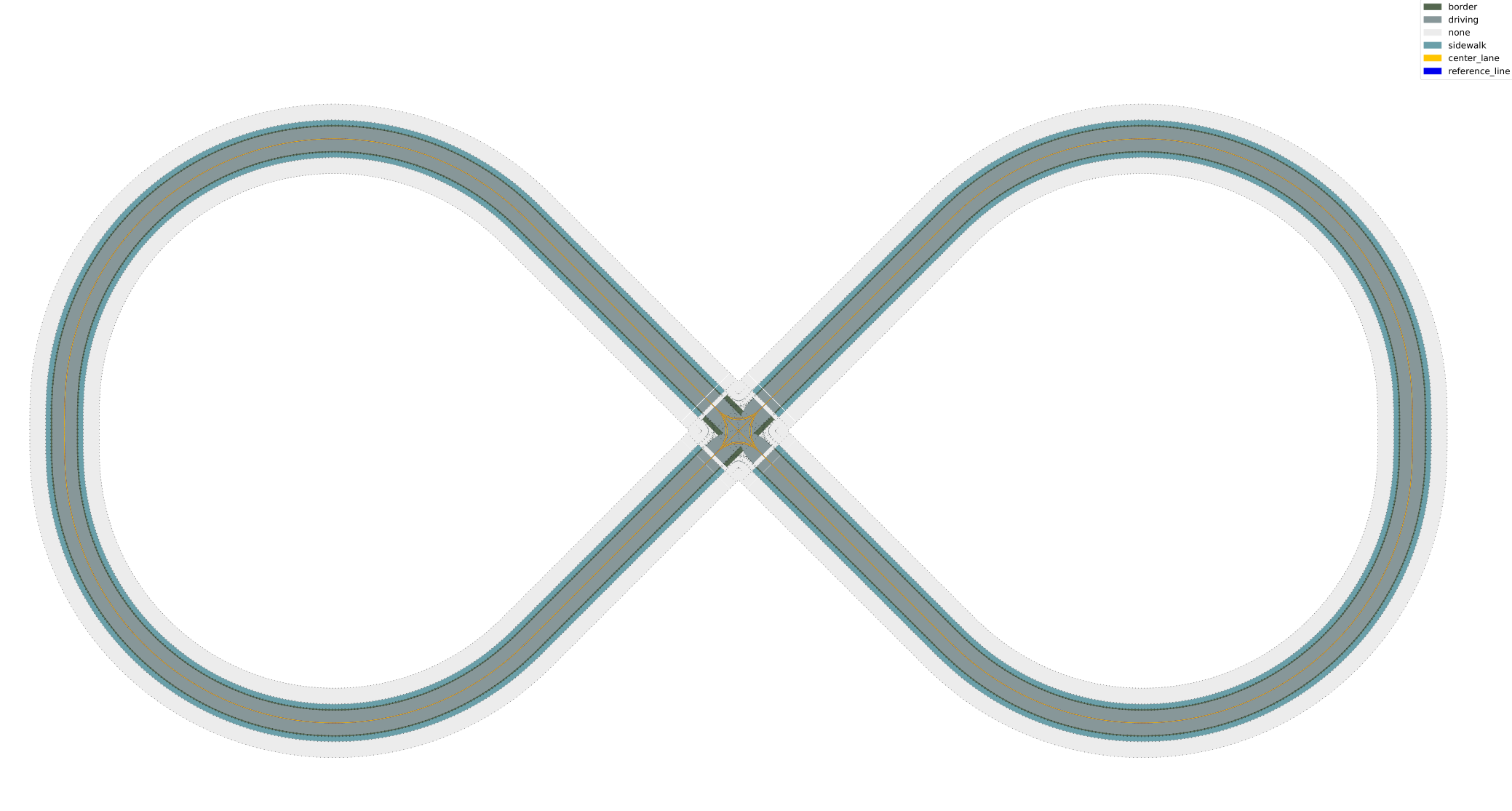
3.4 成品
这里给出在线工具https://odrviewer.io/以及我们绘制的结果。
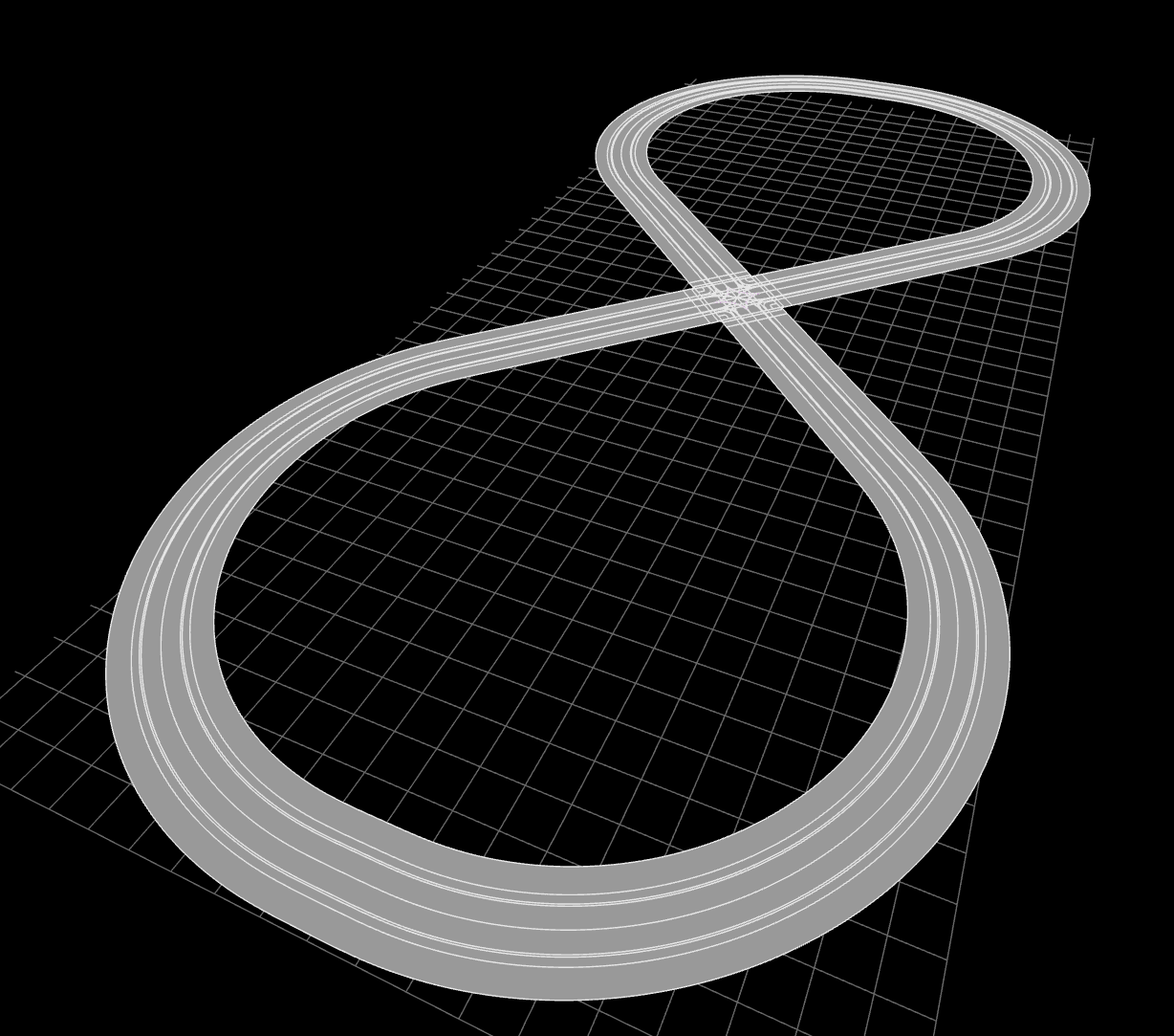
这里需要回答一个关键的问题,既然在线工具已经可以实现绘制,为什么要重复造轮子呢?我们需要注意,在线工具是不开源的,很多情况下我们不仅需要可视化,更多时候需要进一步的开发,因此有必要了解技术细节,了解其来龙去脉。
项目代码已开源:https://github.com/skx6/parse-and-visualize-xodr/tree/main,读者可以据此进行车道可视化和后续计算。
者自知才疏学浅,难免疏漏与谬误,若有高见,请不吝赐教,笔者将不胜感激!
softargmax
2024年4月7日


 3万+
3万+

 被折叠的 条评论
为什么被折叠?
被折叠的 条评论
为什么被折叠?
 到【灌水乐园】发言


