


推荐一个自动控制小车开源项目:本文结合老王自动驾驶控制算法第五讲的离散LQR进行学习复盘
Inverted Pendulum Control — PythonRobotics documentation

-
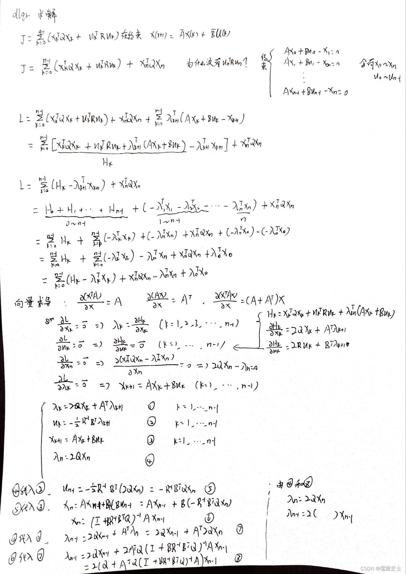
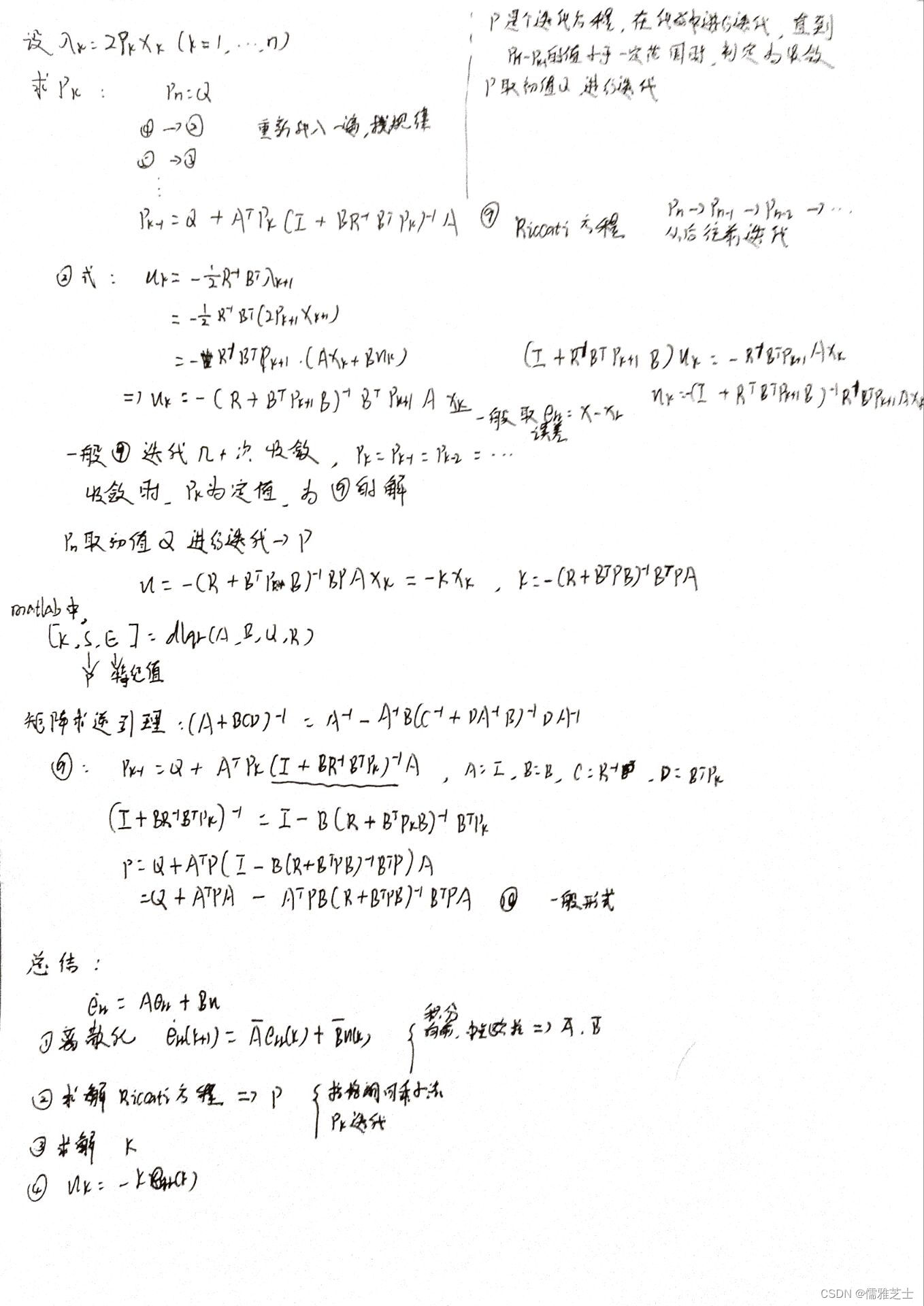
dlqr原理(老王的拉格朗日乘子法)

- 由于函数较多,写了一个框架方便理解。

- 代码如下代,内附官方和自己的注释:
"""
Inverted Pendulum LQR control
author: Trung Kien - letrungkien.k53.hut@gmail.com
"""

import math
import time

import matplotlib.pyplot as plt
import numpy as np
from numpy.linalg import inv, eig

# Model parameters

l_bar = 2.0  # length of bar
M = 1.0  # [kg]
m = 0.3  # [kg]
g = 9.8  # [m/s^2]

nx = 4  # number of state
nu = 1  # number of input
Q = np.diag([0.0, 1.0, 1.0, 0.0])  # state cost matrix。返回所给元素组成的对角矩阵
R = np.diag([0.01])  # input cost matrix

delta_t = 0.1  # time tick [s]
sim_time = 5.0  # simulation time [s]

show_animation = True #一个为真的变量

## 1
def main():
    # x=[x,dot_x,seta,dot_seita]
    x0 = np.array([
        [0.0],
        [0.0],
        [0.3],#倾斜角
        [0.0]
    ])

    # x = np.copy(x0)
    x = x0
    time = 0.0

    while sim_time > time:
        time += delta_t

        # calc control input
        u = lqr_control(x)#调用函数

        # simulate inverted pendulum cart
        x = simulation(x, u)#调用函数

        if show_animation:
            plt.clf()#Clear the current figure.清楚每一帧的动画
            print("X[0]:",x[0])
            # print("X:",x)
            px = float(x[0])#将一个字符串或数字转换为浮点数。输出位置
            theta = float(x[2])#输出角度
            plot_cart(px, theta)#调用函数
            plt.xlim([-5.0, 2.0])
            plt.pause(0.001)#暂停间隔

    print("Finish")
    print(f"x={float(x[0]):.2f} [m] , theta={math.degrees(x[2]):.2f} [deg]")
    if show_animation:
        plt.show()


## 2
def simulation(x, u):
    '''
    调整X
    '''
    A, B = get_model_matrix()#调用函数,得到AB矩阵

    x = A @ x + B @ u#矩阵乘法,必须声明numpy

    return x


## 3
def solve_DARE(A, B, Q, R, maxiter=150, eps=0.01):
    """
    Solve a discrete time_Algebraic Riccati equation (DARE)求得离散时间黎卡提方程的解 矩阵P
    """
    P = Q#初始化

    for i in range(maxiter):
        #矩阵P进行迭代,4×4的矩阵
        Pn = A.T @ P @ A - A.T @ P @ B @ inv(R + B.T @ P @ B) @ B.T @ P @ A + Q
        # print("Pn:",Pn)
        #矩阵P收敛时,退出迭代循环
        # print("abs(Pn - P).max:",abs(Pn - P).max(),i)
        # print("Pn - P:",Pn - P,i)
        if (abs(Pn - P)).max() < eps:
            break
        P = Pn

    return Pn#收敛的矩阵P


    # P = Q
    # for i in range(50):
    #     Pn = A.T @ P @ A - A.T @ P @ B @ inv(R + B.T @ P @ B ) @ B.T @ P @ A +Q
    #     # print("Pn:",Pn)
    #     # print("P:",P)
    #     if (abs(Pn - P)).max() < 0.01:
    #         break
    # return Pn

## 4
def dlqr(A, B, Q, R):
    """
    Solve the discrete time lqr controller.
    x[k+1] = A x[k] + B u[k]
    cost = sum x[k].T*Q*x[k] + u[k].T*R*u[k]
    # ref Bertsekas, p.151
    """

    # first, try to solve the ricatti equation
    #先求解迭代后收敛的矩阵P
    P = solve_DARE(A, B, Q, R)

    # compute the LQR gain
    #计算矩阵K,u=-KX
    K = inv(B.T @ P @ B + R) @ (B.T @ P @ A)#u=-kx的k

    eigVals, eigVecs = eig(A - B @ K)#计算方阵的特征值和右特征向量

    return K, P, eigVals


## 5
def lqr_control(x):
    '''
    得到输入u
    '''
    A, B = get_model_matrix()
    start = time.time()
    K, _, _ = dlqr(A, B, Q, R)
    u = -K @ x
    elapsed_time = time.time() - start
    print(f"calc time:{elapsed_time:.6f} [sec]")
    return u#返回输入u


## 6
def get_numpy_array_from_matrix(x):
    """
    get build-in list from matrix,将多维数组降为一维
    """
    return np.array(x).flatten()#将多维数组降为一维


## 7
def get_model_matrix():
    '''
    更新离散过程中的矩阵A、B
    '''
    A = np.array([
        [0.0, 1.0, 0.0, 0.0],
        [0.0, 0.0, m * g / M, 0.0],
        [0.0, 0.0, 0.0, 1.0],
        [0.0, 0.0, g * (M + m) / (l_bar * M), 0.0]
    ])

    # A = np.eye(nx) + delta_t * A#单位矩阵+△t*A,收敛速度慢
    A = inv(np.eye(4) - A *1/2 * delta_t) @ (np.eye(4) + A *1/2 * delta_t)#收敛更快

    B = np.array([
        [0.0],
        [1.0 / M],
        [0.0],
        [1.0 / (l_bar * M)]
    ])
    B = delta_t * B

    return A, B


## 8
def flatten(a):
    """
    将多维数组降为一维
    """
    return np.array(a).flatten()


## 9
def plot_cart(xt, theta):#xt:小球位置
    """
    画图
    """
    cart_w = 1.0#马车宽
    cart_h = 0.5#马车高
    radius = 0.1#马车轮半径

    cx = np.array([-cart_w / 2.0, cart_w / 2.0, cart_w /2.0, -cart_w / 2.0, -cart_w / 2.0])#马车顶点x坐标矩阵,闭合图形的顶点
    cy = np.array([0.0, 0.0, cart_h, cart_h, 0.0])#马车顶点y坐标
    cy += radius * 2.0#加轮高

    cx = cx + xt#调整马车位置,以球心坐标为基点变化

    bx = np.array([0.0, l_bar * math.sin(-theta)])#球心的x坐标
    bx += xt
    by = np.array([cart_h, l_bar * math.cos(-theta) + cart_h])#球心的y坐标
    by += radius * 2.0

    ##画车轮的圆
    #np.arange返回一个有终点和起点的固定步长的排列,第一个参数为起点,第二个参数为终点,第三个参数为步长
    angles = np.arange(0.0, math.pi * 2.0, math.radians(3.0))#math.radians()返回弧度制。离散化
    #每一步的x、y随球的旋转弧度变化
    ox = np.array([radius * math.cos(a) for a in angles])#np.array()的作用就是按照一定要求将object转换为数组
    oy = np.array([radius * math.sin(a) for a in angles])
    #右轮
    rwx = np.copy(ox) + cart_w / 4.0 + xt#右轮位置 = 离散矩阵 + 0.25 + 球位置
    rwy = np.copy(oy) + radius#离散矩阵
    #左轮
    lwx = np.copy(ox) - cart_w / 4.0 + xt
    lwy = np.copy(oy) + radius

    ##画球
    wx = np.copy(ox) + bx[-1]
    wy = np.copy(oy) + by[-1]

    plt.plot(flatten(cx), flatten(cy), "-b")#马车
    plt.plot(flatten(bx), flatten(by), "-k")#摆杆
    plt.plot(flatten(rwx), flatten(rwy), "-k")#右轮
    plt.plot(flatten(lwx), flatten(lwy), "-k")#左球
    plt.plot(flatten(wx), flatten(wy), "-k")#球
    plt.title(f"x: {xt:.2f} , theta: {math.degrees(theta):.2f}")

    # for stopping simulation with the esc key.
    plt.gcf().canvas.mpl_connect(
        'key_release_event',
        lambda event: [exit(0) if event.key == 'escape' else None])

    plt.axis("equal")


if __name__ == '__main__':
    main()
自己根据老王的dlqr推导过程,仿着开源代码修改了自己的代码,由于开源代码有些地方较为冗长,自己在函数顺序方面做了改进,图像plot部分未做修改
import math
import time

import matplotlib.pyplot as plt
import numpy as np
from numpy.linalg import inv, eig

l_bar = 2.0  # length of bar
M = 1.0  # [kg]
m = 0.3  # [kg]
g = 9.8  # [m/s^2]

nx = 4  # number of state
nu = 1  # number of input
Q = np.diag([0.0, 1.0, 1.0, 0.0])  # state cost matrix。返回所给元素组成的对角矩阵
R = np.diag([0.01])  # input cost matrix

delta_t = 0.1  # time tick [s]
sim_time = 5.0  # simulation time [s]


show_animation = True #一个为真的变量

#主函数√
def  main():
    time = 0.0
    X0 = np.array([
        [0.0],
        [0.0],
        [0.3],
        [0.0]
    ])

    X = X0
    while sim_time > time:
        time += delta_t

        A,B = get_A_B()
        P = get_P(A,B,R,Q)
        K = get_K(A,B,R,P)
        u = get_u(K, X)
        X = A @ X + B @ u

        if show_animation:
            plt.clf()#Clear the current figure.清楚每一帧的动画
            px = float(X[0])#将一个字符串或数字转换为浮点数。输出位置
            theta = float(X[2])#输出角度
            plot_cart(px, theta)#调用函数
            plt.xlim([-5.0, 5.0])
            plt.pause(0.001)#暂停间隔
    print("Finish")
    print(f"x={float(X[0]):.2f} [m] , theta={math.degrees(X[2]):.2f} [deg]")
    if show_animation:
        plt.show()


#获取p矩阵√
def get_P(A,B,R,Q):
    P = Q
    # Pn = A.T @ P @ A - A.T @ P @ B @ inv(R + B.T @ P @ B ) @ B.T @ P @ A +Q
    # print("Pn:",Pn)
    for i in range(150):
        Pn = A.T @ P @ A - A.T @ P @ B @ inv(R + B.T @ P @ B ) @ B.T @ P @ A +Q
        # print("Pn:",Pn)
        # print("P:",P)
        if (abs(Pn - P)).max()< 0.01:
            break
        P = Pn

    return Pn


#获取A,B√√√
def get_A_B():
    A0 = np.array([
        [0.0, 1.0, 0.0, 0.0],
        [0.0, 0.0, m * g / M, 0.0],
        [0.0, 0.0, 0.0, 1.0],
        [0.0, 0.0, g * (M + m) / (l_bar * M), 0.0]
    ])

    B0 = np.array([
        [0.0],
        [1.0 / M],
        [0.0],
        [1.0 / (l_bar * M)]
    ])

    A = inv(np.eye(4) - A0 *1/2 * delta_t) @ (np.eye(4) + A0 *1/2 * delta_t)
    B = B0 * delta_t

    return A,B


#获取K矩阵
def get_K(A,B,R,P):
    K = inv(B.T @ P @ B + R) @(B.T @ P @ A)
    return K


# 获取输入u
def get_u(K, X):
    u = -1 * K @ X
    return u


## 8
def flatten(a):
    """
    将多维数组降为一维
    """
    return np.array(a).flatten()


def plot_cart(xt, theta):
    """
    画图
    """
    cart_w = 1.0
    cart_h = 0.5
    radius = 0.1

    cx = np.array([-cart_w / 2.0, cart_w / 2.0, cart_w /
                   2.0, -cart_w / 2.0, -cart_w / 2.0])
    cy = np.array([0.0, 0.0, cart_h, cart_h, 0.0])
    cy += radius * 2.0

    cx = cx + xt

    bx = np.array([0.0, l_bar * math.sin(-theta)])
    bx += xt
    by = np.array([cart_h, l_bar * math.cos(-theta) + cart_h])
    by += radius * 2.0

    angles = np.arange(0.0, math.pi * 2.0, math.radians(3.0))
    ox = np.array([radius * math.cos(a) for a in angles])
    oy = np.array([radius * math.sin(a) for a in angles])

    rwx = np.copy(ox) + cart_w / 4.0 + xt
    rwy = np.copy(oy) + radius
    lwx = np.copy(ox) - cart_w / 4.0 + xt
    lwy = np.copy(oy) + radius

    wx = np.copy(ox) + bx[-1]
    wy = np.copy(oy) + by[-1]

    plt.plot(flatten(cx), flatten(cy), "-b")
    plt.plot(flatten(bx), flatten(by), "-k")
    plt.plot(flatten(rwx), flatten(rwy), "-k")
    plt.plot(flatten(lwx), flatten(lwy), "-k")
    plt.plot(flatten(wx), flatten(wy), "-k")
    plt.title(f"x: {xt:.2f} , theta: {math.degrees(theta):.2f}")

    # for stopping simulation with the esc key.
    plt.gcf().canvas.mpl_connect(
        'key_release_event',
        lambda event: [exit(0) if event.key == 'escape' else None])

    plt.axis("equal")


if __name__ == '__main__':
    main()


 948
948


 被折叠的 条评论
为什么被折叠?
被折叠的 条评论
为什么被折叠?
 到【灌水乐园】发言


