


https://github.com/smorabit/hdWGCNA
官方教程
https://smorabit.github.io/hdWGCNA/articles/basic_tutorial.html
hdWGCNA in single-cell data
This tutorial covers the basics of using hdWGCNA to perform co-expression network analysis on single-cell data. Here, we demonstrate hdWGCNA using a processed single-nucleus RNA-seq (snRNA-seq) dataset of human cortical samples from this publication. This dataset has already been fully processed using a standard single-cell transcritpomics analysis pipeline such as Seurat or Scanpy. If you would like to follow this tutorial using your own dataset, you first need to satisfy the following prerequisites:
- A single-cell or single-nucleus transcriptomics dataset in Seurat format.
- Normalize the gene expression matrix NormalizeData.
- Identify highly variable genes VariableFeatures.
- Scale the normalized expression data ScaleData
- Perform dimensionality reduction RunPCA and batch correction if needed RunHarmony.
- Non-linear dimensionality reduction RunUMAP for visualizations.
- Group cells into clusters (FindNeighbors and FindClusters).
An example of running the prerequisite data processing steps can be found in the Seurat Guided Clustering Tutorial.
Additionally, there are a lot of WGCNA-specific terminology and acronyms, which are all clarified in this table.
Download the tutorial data
For the purpose of this tutorial, we provide a processed Seurat object of the control human brains from the Zhou et al 2020 study.
wget https://swaruplab.bio.uci.edu/public_data/Zhou_2020.rdsDownload not working?
Load the dataset and required libraries
First we will load the single-cell dataset and the required R libraries for this tutorial.
# single-cell analysis package
library(Seurat)

# plotting and data science packages
library(tidyverse)
library(cowplot)
library(patchwork)

# co-expression network analysis packages:
library(WGCNA)
library(hdWGCNA)

# using the cowplot theme for ggplot
theme_set(theme_cowplot())

# set random seed for reproducibility
set.seed(12345)

# load the Zhou et al snRNA-seq dataset
seurat_obj <- readRDS('Zhou_2020.rds')
Here we will plot the UMAP colored by cell type just to check that we have loaded the data correctly, and to make sure that we have grouped cells into clusters and cell types.
p <- DimPlot(seurat_obj, group.by='cell_type', label=TRUE) +
   umap_theme() + ggtitle('Zhou et al Control Cortex') + NoLegend()

p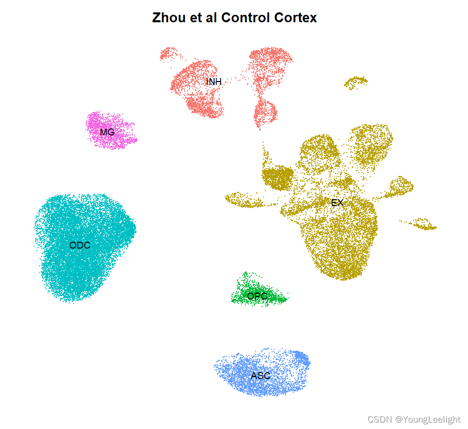
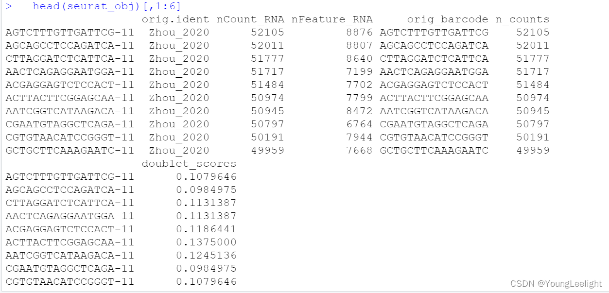
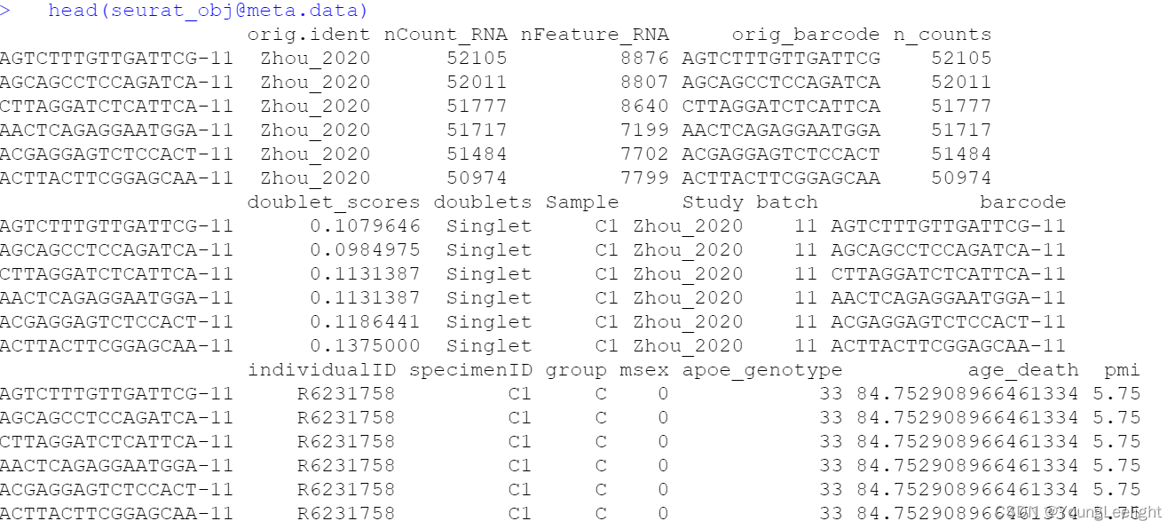
> head(seurat_obj@meta.data)
orig.ident nCount_RNA nFeature_RNA orig_barcode n_counts
AGTCTTTGTTGATTCG-11 Zhou_2020 52105 8876 AGTCTTTGTTGATTCG 52105
AGCAGCCTCCAGATCA-11 Zhou_2020 52011 8807 AGCAGCCTCCAGATCA 52011
CTTAGGATCTCATTCA-11 Zhou_2020 51777 8640 CTTAGGATCTCATTCA 51777
AACTCAGAGGAATGGA-11 Zhou_2020 51717 7199 AACTCAGAGGAATGGA 51717
ACGAGGAGTCTCCACT-11 Zhou_2020 51484 7702 ACGAGGAGTCTCCACT 51484
ACTTACTTCGGAGCAA-11 Zhou_2020 50974 7799 ACTTACTTCGGAGCAA 50974
doublet_scores doublets Sample Study batch barcode
AGTCTTTGTTGATTCG-11 0.1079646 Singlet C1 Zhou_2020 11 AGTCTTTGTTGATTCG-11
AGCAGCCTCCAGATCA-11 0.0984975 Singlet C1 Zhou_2020 11 AGCAGCCTCCAGATCA-11
CTTAGGATCTCATTCA-11 0.1131387 Singlet C1 Zhou_2020 11 CTTAGGATCTCATTCA-11
AACTCAGAGGAATGGA-11 0.1131387 Singlet C1 Zhou_2020 11 AACTCAGAGGAATGGA-11
ACGAGGAGTCTCCACT-11 0.1186441 Singlet C1 Zhou_2020 11 ACGAGGAGTCTCCACT-11
ACTTACTTCGGAGCAA-11 0.1375000 Singlet C1 Zhou_2020 11 ACTTACTTCGGAGCAA-11
individualID specimenID group msex apoe_genotype age_death pmi
AGTCTTTGTTGATTCG-11 R6231758 C1 C 0 33 84.752908966461334 5.75
AGCAGCCTCCAGATCA-11 R6231758 C1 C 0 33 84.752908966461334 5.75
CTTAGGATCTCATTCA-11 R6231758 C1 C 0 33 84.752908966461334 5.75
AACTCAGAGGAATGGA-11 R6231758 C1 C 0 33 84.752908966461334 5.75
ACGAGGAGTCTCCACT-11 R6231758 C1 C 0 33 84.752908966461334 5.75
ACTTACTTCGGAGCAA-11 R6231758 C1 C 0 33 84.752908966461334 5.75
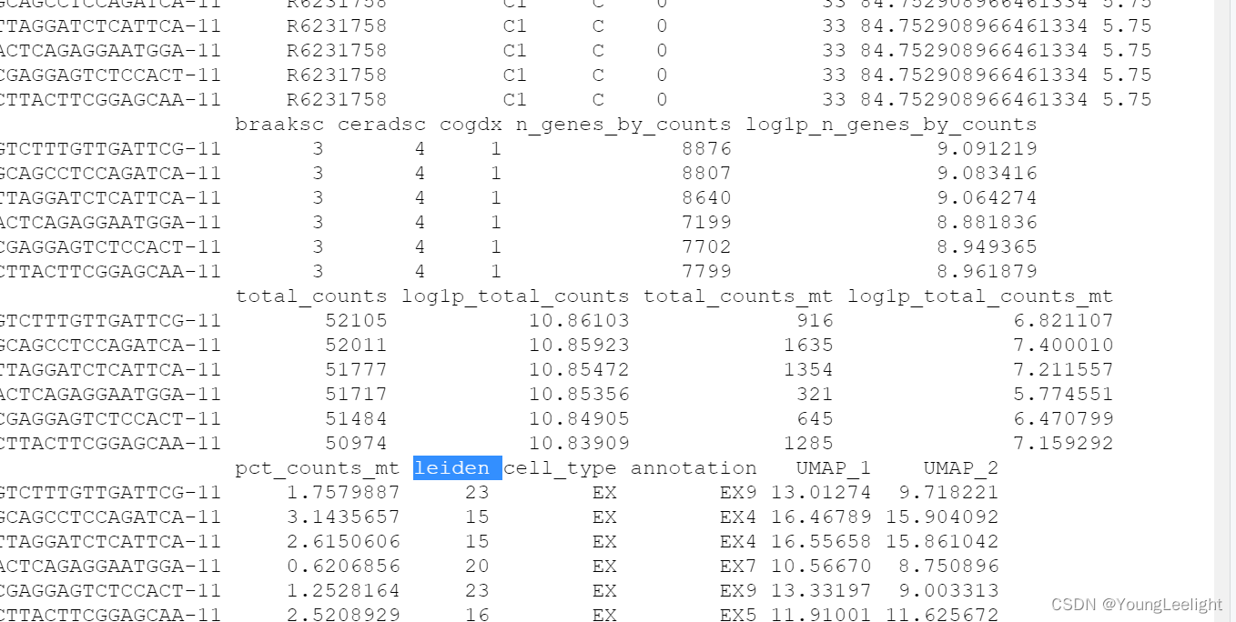
braaksc ceradsc cogdx n_genes_by_counts log1p_n_genes_by_counts
AGTCTTTGTTGATTCG-11 3 4 1 8876 9.091219
AGCAGCCTCCAGATCA-11 3 4 1 8807 9.083416
CTTAGGATCTCATTCA-11 3 4 1 8640 9.064274
AACTCAGAGGAATGGA-11 3 4 1 7199 8.881836
ACGAGGAGTCTCCACT-11 3 4 1 7702 8.949365
ACTTACTTCGGAGCAA-11 3 4 1 7799 8.961879
total_counts log1p_total_counts total_counts_mt log1p_total_counts_mt
AGTCTTTGTTGATTCG-11 52105 10.86103 916 6.821107
AGCAGCCTCCAGATCA-11 52011 10.85923 1635 7.400010
CTTAGGATCTCATTCA-11 51777 10.85472 1354 7.211557
AACTCAGAGGAATGGA-11 51717 10.85356 321 5.774551
ACGAGGAGTCTCCACT-11 51484 10.84905 645 6.470799
ACTTACTTCGGAGCAA-11 50974 10.83909 1285 7.159292
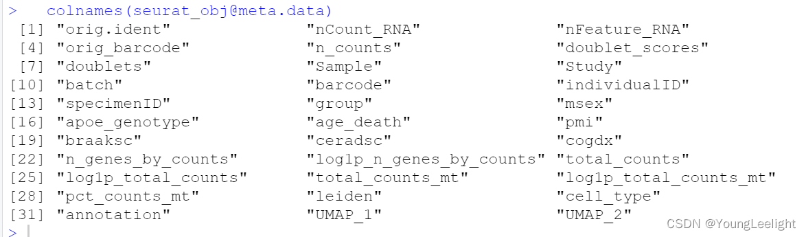
pct_counts_mt leiden cell_type annotation UMAP_1 UMAP_2
AGTCTTTGTTGATTCG-11 1.7579887 23 EX EX9 13.01274 9.718221
AGCAGCCTCCAGATCA-11 3.1435657 15 EX EX4 16.46789 15.904092
CTTAGGATCTCATTCA-11 2.6150606 15 EX EX4 16.55658 15.861042
AACTCAGAGGAATGGA-11 0.6206856 20 EX EX7 10.56670 8.750896
ACGAGGAGTCTCCACT-11 1.2528164 23 EX EX9 13.33197 9.003313
ACTTACTTCGGAGCAA-11 2.5208929 16 EX EX5 11.91001 11.625672Set up Seurat object for WGCNA
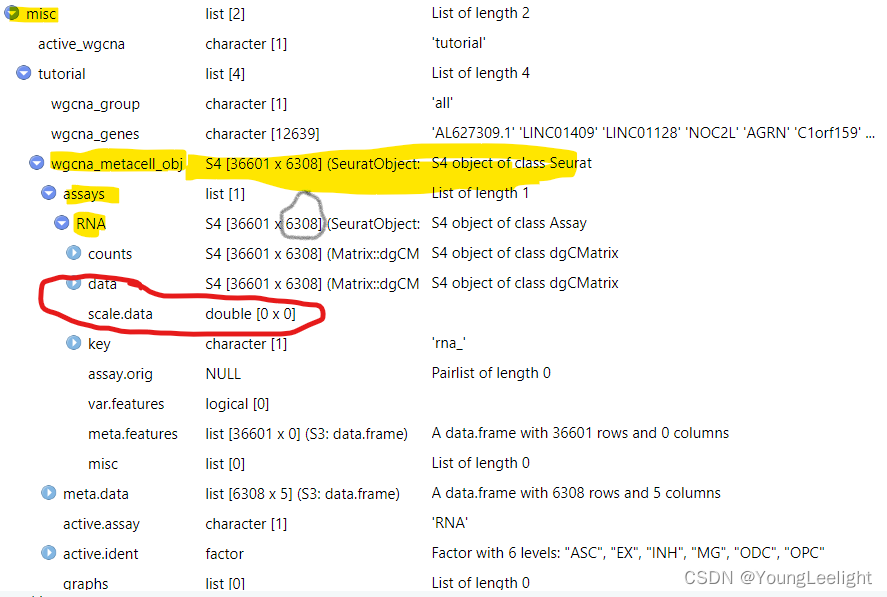
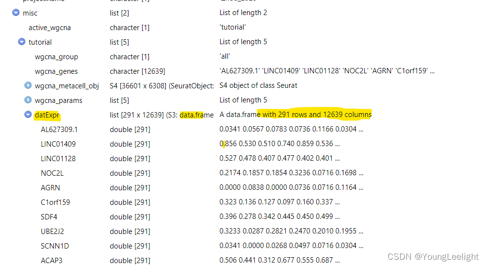
Before running hdWGCNA, we first have to set up the Seurat object. Most of the information computed by hdWGCNA is stored in the Seurat object’s @misc slot. A single Seurat object can hold multiple hdWGCNA experiments, for example representing different cell types in the same single-cell dataset. Notably, since we consider hdWGCNA to be a downstream data analysis step, we do not support subsetting the Seurat object after SetupForWGCNA has been run.
Here we will set up the Seurat object using the SetupForWGCNA function, specifying the name of the hdWGNCA experiment. This function also selects the genes that will be used for WGCNA. The user can select genes using three different approaches using the gene_select parameter:
variable: use the genes stored in the Seurat object’sVariableFeatures.fraction: use genes that are expressed in a certain fraction of cells for in the whole dataset or in each group of cells, specified bygroup.by.custom: use genes that are specified in a custom list.
In this example, we will select genes that are expressed in at least 5% of cells in this dataset, and we will name our hdWGCNA experiment “tutorial”.
seurat_obj <- SetupForWGCNA(
  seurat_obj,
  gene_select = "fraction", # the gene selection approach
  fraction = 0.05, # fraction of cells that a gene needs to be expressed in order to be included
  wgcna_name = "tutorial" # the name of the hdWGCNA experiment
)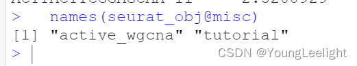
> names(seurat_obj@misc)
[1] "active_wgcna" "tutorial"
> dim(seurat_obj)
[1] 36601 36671
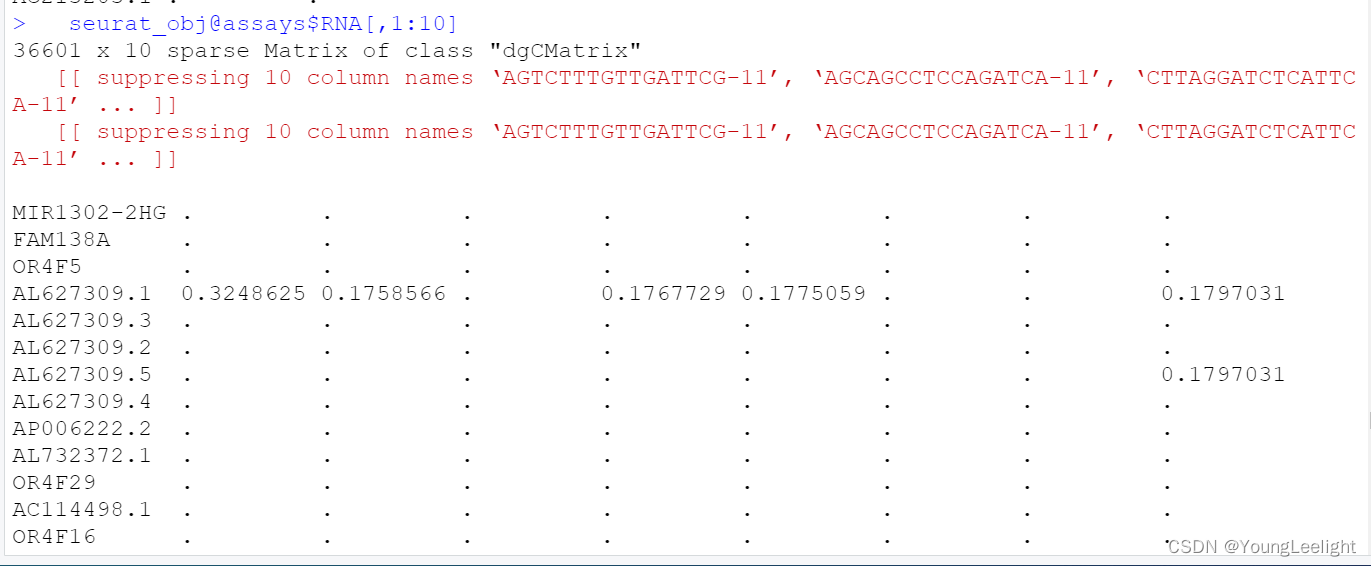
> dim(seurat_obj@assays$RNA)
[1] 36601 36671
> dim(seurat_obj@assays$RNA@counts)
[1] 36601 36671
Construct metacells
After we have set up our Seurat object, the first step in running the hdWGCNA pipeine in hdWGCNA is to construct metacells from the single-cell dataset. Briefly, metacells are aggregates of small groups of similar cells originating from the same biological sample of origin. The k-Nearest Neighbors (KNN) algorithm is used to identify groups of similar cells to aggregate, and then the average or summed expression of these cells is computed, thus yielding a metacell gene expression matrix. The sparsity of the metacell expression matrix is considerably reduced when compared to the original expression matrix, and therefore it is preferable to use. We were originally motivated to use metacells in place of the original single cells because correlation network approaches such as WGCNA are sensitive to data sparsity. Furthermore, single-cell epigenomic approaches, such as Cicero, employ a similar metacell aggregation approach prior to constructing co-accessibility networks.
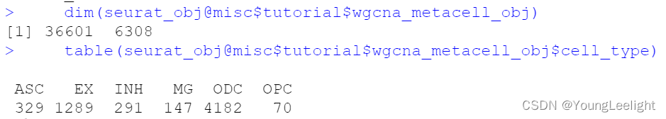
hdWGCNA includes a function MetacellsByGroups to construct metacell expression matrices given a single-cell dataset. This function constructs a new Seurat object for the metacell dataset which is stored internally in the hdWGCNA experiment. The group.by parameter determines which groups metacells will be constructed in. We only want to construct metacells from cells that came from the same biological sample of origin, so it is critical to pass that information to hdWGCNA via the group.by parameter. Additionally, we usually construct metacells for each cell type separately. Thus, in this example, we are grouping by Sample and cell_type to achieve the desired result.
The number of cells to be aggregated k should be tuned based on the size of the input dataset, in general a lower number for k can be used for small datasets. We generally use k values between 20 and 75. The dataset used for this tutorial has 40,039 cells, ranging from 890 to 8,188 in each biological sample, and here we used k=25. The amount of allowable overlap between metacells can be tuned using the max_shared argument.
Note: we have found that the metacell aggregation approach does not yield good results for extremely underrepresented cell types. For example, in this dataset, the brain vascular cells (pericytes and endothelial cells) were the least represented, and we have excluded them from this analysis. MetacellsByGroups has a parameter min_cells to exclude groups that are smaller than a specified number of cells.
Here we construct metacells and normalize the resulting expression matrix using the following code:

# construct metacells  in each group
seurat_obj <- MetacellsByGroups(
  seurat_obj = seurat_obj,
  group.by = c("cell_type", "Sample"), # specify the columns in seurat_obj@meta.data to group by
  k = 25, # nearest-neighbors parameter
  max_shared = 10, # maximum number of shared cells between two metacells
  ident.group = 'cell_type' # set the Idents of the metacell seurat object
)
> names(seurat_obj@misc)
[1] "active_wgcna" "tutorial"
# normalize metacell expression matrix:
seurat_obj <-NormalizeMetacells(seurat_obj)
Optional: Process the Metacell Seurat Object
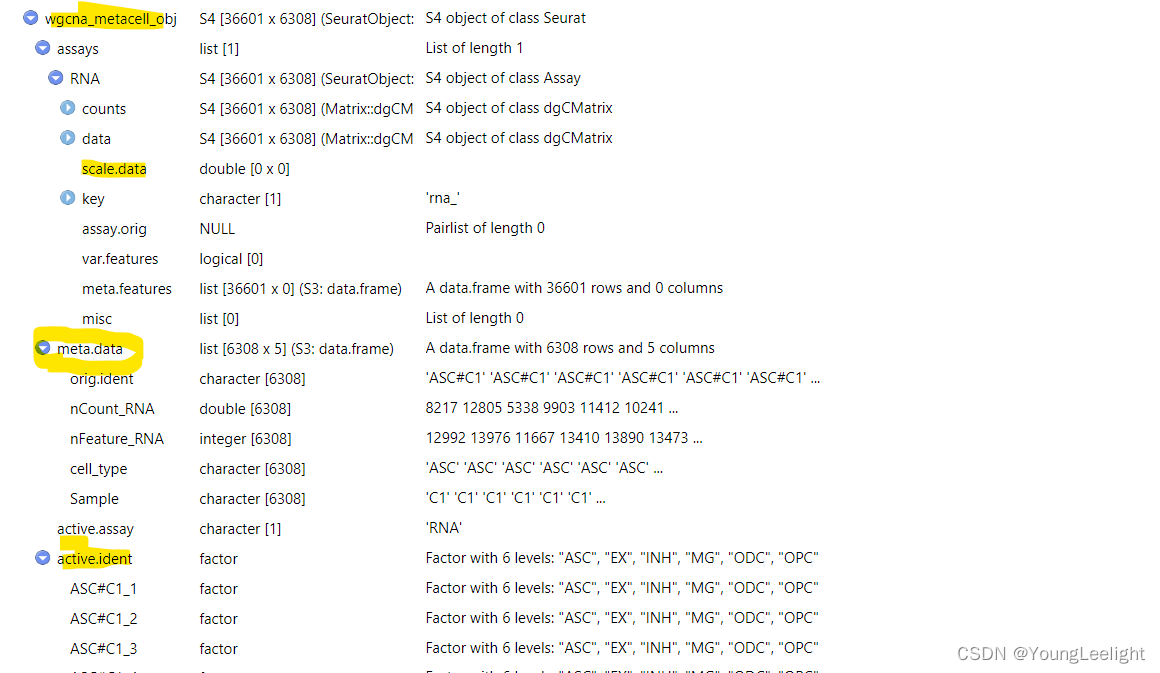
Since we store the Metacell expression information as its own Seurat object, we can run Seurat functions on the metacell data. We can get the metacell object from the hdWGCNA experiment using GetMetacellObject.
metacell_obj <- GetMetacellObject(seurat_obj) 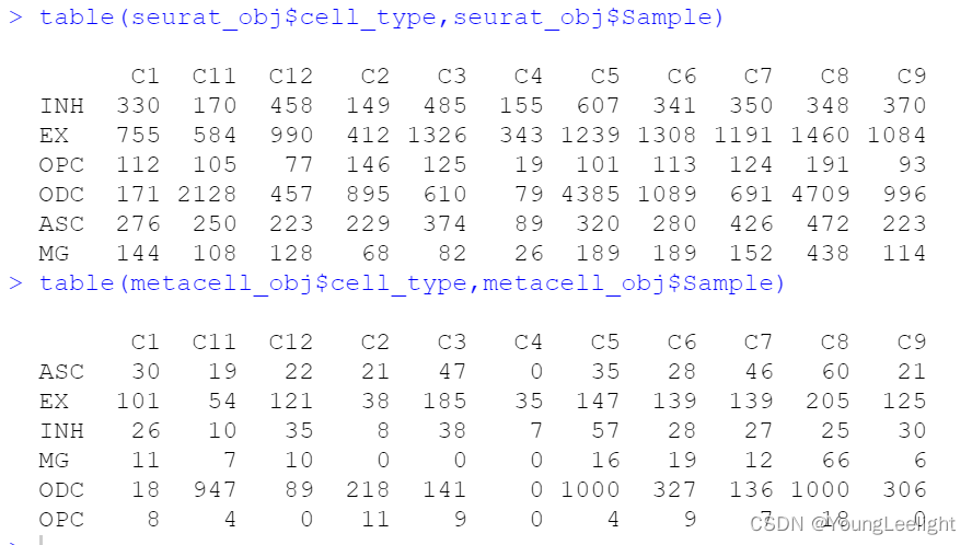
Additionally, we have included a few wrapper functions to apply the Seurat workflow to the metacell object within the hdWGCNA experiment. Here we apply these wrapper functions to process the metacell object and visualize the aggregated expression profiles in two dimensions with UMAP.
seurat_obj <- NormalizeMetacells(seurat_obj)
 seurat_obj<-FindVariableFeatures(seurat_obj)#我自己加的一个步骤本来没有的
seurat_obj <- ScaleMetacells(seurat_obj, features=VariableFeatures(seurat_obj))


seurat_obj <- RunPCAMetacells(seurat_obj, features=VariableFeatures(seurat_obj))
seurat_obj <- RunHarmonyMetacells(seurat_obj, group.by.vars='Sample')
seurat_obj <- RunUMAPMetacells(seurat_obj, reduction='harmony', dims=1:15)


p1 <- DimPlotMetacells(seurat_obj, group.by='cell_type') + umap_theme() + ggtitle("Cell Type")
p2 <- DimPlotMetacells(seurat_obj, group.by='Sample') + umap_theme() + ggtitle("Sample")

p1 | p2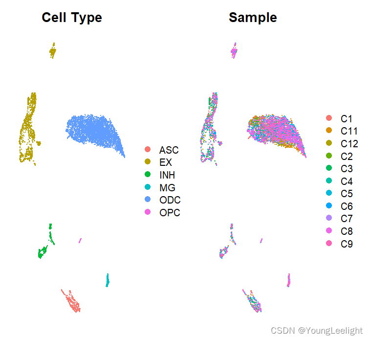
Co-expression network analysis
In this section we discuss how to perform co-expression network analysis with hdWGNCA on the inhibitory neuron (INH) cells in our example dataset.
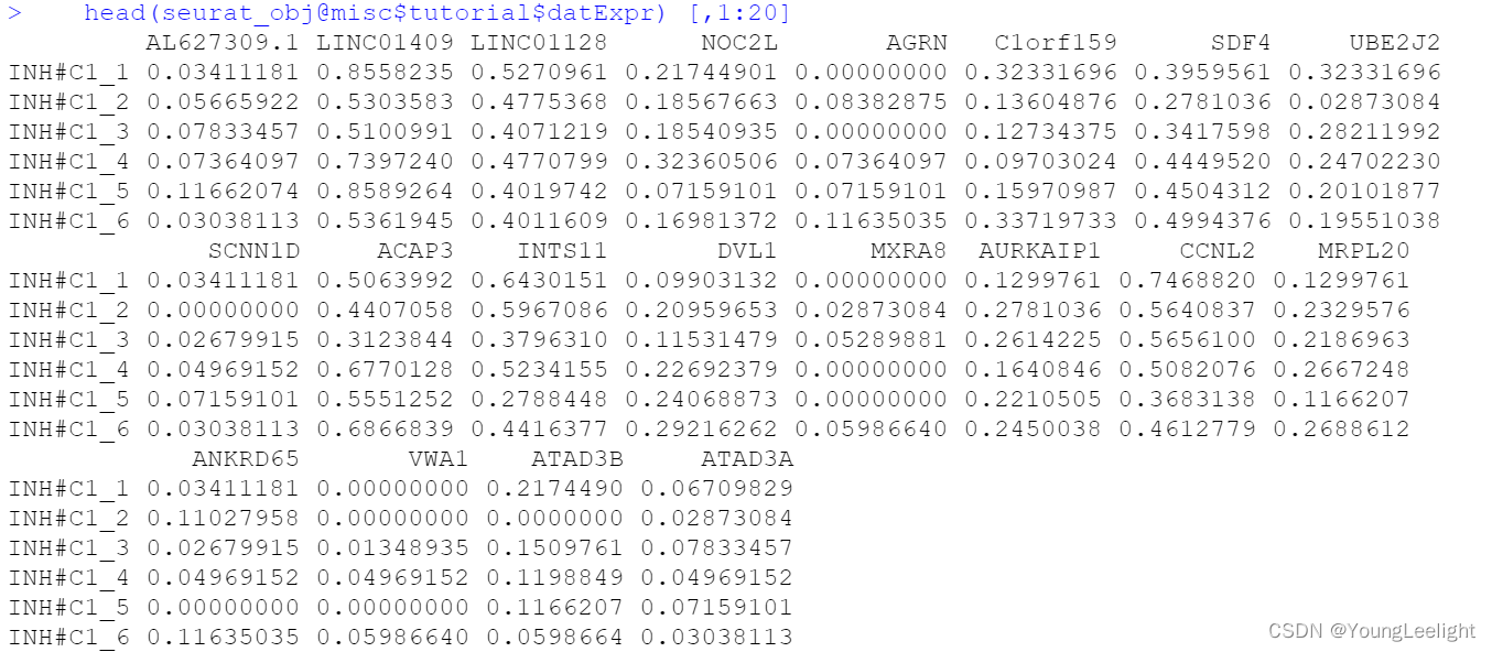
Set up the expression matrix
Here we specify the expression matrix that we will use for network analysis. Since We only want to include the inhibitory neurons, so we have to subset our expression data prior to constructing the network. hdWGCNA includes the SetDatExpr function to store the transposed expression matrix for a given group of cells that will be used for downstream network analysis. The metacell expression matrix is used by default (use_metacells=TRUE), but hdWGCNA does allow for the single-cell expression matrix to be used if desired.. This function allows the user to specify which slot to take the expression matrix from, for example if the user wanted to apply SCTransform normalization instead of NormalizeData.
seurat_obj <- SetDatExpr(
  seurat_obj,
  group_name = "INH", # the name of the group of interest in the group.by column
  group.by='cell_type', # the metadata column containing the cell type info. This same column should have also been used in MetacellsByGroups
  assay = 'RNA', # using RNA assay
  slot = 'data' # using normalized data
)
Selecting more than one group
Suppose that you want to perform co-expression network analysis on more than one cell type or cluster simultaneously. SetDatExpr can be run with slighly different settings to achieve the desired result by passing a character vector to the group_name parameter.
seurat_obj <- SetDatExpr(
  seurat_obj,
  group_name = c("INH", "EX"),
  group.by='cell_type'
)
这里去了INH meta细胞
Select soft-power threshold
Next we will select the “soft power threshold”. This is an extremely important step in the hdWGNCA pipleine (and for vanilla WGCNA). hdWGCNA constructs a gene-gene correlation adjacency matrix to infer co-expression relationships between genes. The correlations are raised to a power to reduce the amount of noise present in the correlation matrix, thereby retaining the strong connections and removing the weak connections. Therefore, it is critical to determine a proper value for the soft power threshold.
We include a function TestSoftPowers to perform a parameter sweep for different soft power thresholds. This function helps us to guide our choice in a soft power threshold for constructing the co-expression network by inspecting the resulting network topology for different power values. The co-expression network should have a scale-free topology, therefore the TestSoftPowers function models how closely the co-expression network resembles a scale-free graph at different soft power thresholds. Furthermore, we include a function PlotSoftPowers to visualize the results of the parameter sweep.
The following code performs the parameter sweep and outputs a summary figure.
# Test different soft powers:
seurat_obj <- TestSoftPowers(
  seurat_obj,use_metacells = TRUE,
  networkType = 'signed' # you can also use "unsigned" or "signed hybrid"
)

# plot the results:
plot_list <- PlotSoftPowers(seurat_obj)

# assemble with patchwork
wrap_plots(plot_list, ncol=2)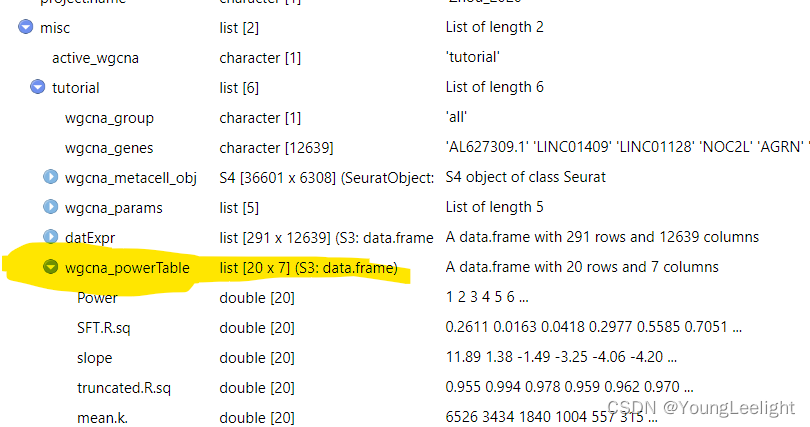
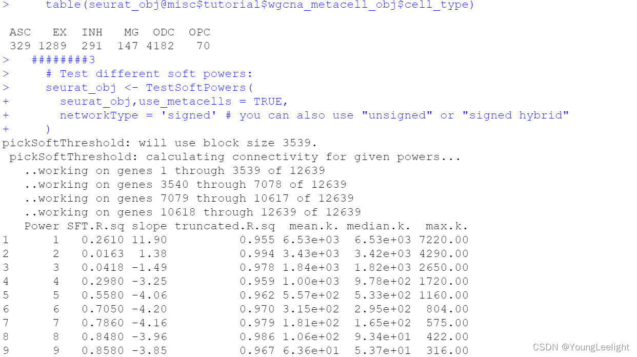
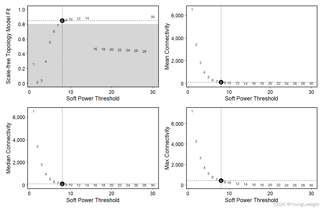
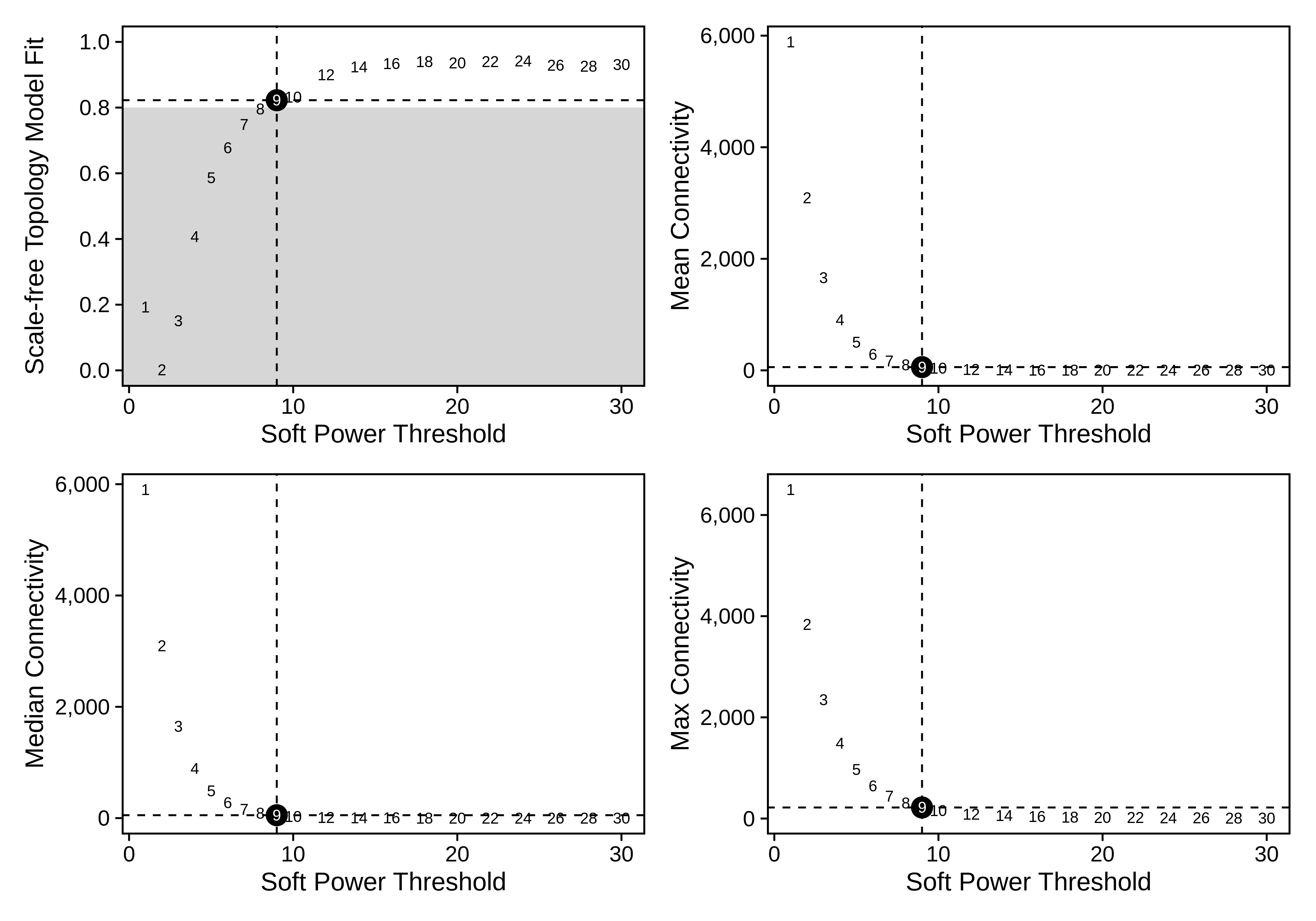
The general guidance for WGCNA and hdWGCNA is to pick the lowest soft power threshold that has a Scale Free Topology Model Fit greater than or equal to 0.8, so in this case we would select our soft power threshold as 9. Later on, the ConstructNetwork will automatically select the soft power threshold if the user does not provide one.
Tthe output table from the parameter sweep is stored in the hdWGCNA experiment and can be accessed using the GetPowerTable function for further inspection:
power_table <- GetPowerTable(seurat_obj)
head(power_table)
> View(seurat_obj)
> View(seurat_obj)
>     power_table <- GetPowerTable(seurat_obj)
>     head(power_table)
  Power   SFT.R.sq     slope truncated.R.sq   mean.k. median.k.    max.k.
1     1 0.26110351 11.889729      0.9546294 6525.7417 6532.2923 7219.7053
2     2 0.01631495  1.375111      0.9935408 3434.0090 3421.8601 4293.1289
3     3 0.04178826 -1.487314      0.9784280 1840.1686 1817.2352 2651.0575
4     4 0.29769630 -3.249674      0.9588046 1003.7962  978.3657 1719.7194
5     5 0.55846894 -4.060086      0.9617106  557.3639  533.2201 1157.0353
6     6 0.70513240 -4.195496      0.9696135  315.0681  295.1368  804.1011
Construct co-expression network
We now have everything that we need to construct our co-expression network. Here we use the hdWGCNA function ConstructNetwork, which calls the WGCNA function blockwiseConsensusModules under the hood. This function has quite a few parameters to play with if you are an advanced user, but we have selected default parameters that work well with many single-cell datasets. The parameters for blockwiseConsensusModules can be passed directly to ConstructNetwork with the same parameter names.
The following code construtcts the co-expression network using the soft power threshold selected above:
# construct co-expression network:
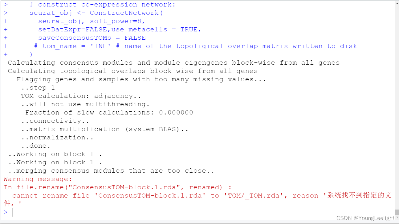
seurat_obj <- ConstructNetwork(
seurat_obj, soft_power=9,
setDatExpr=FALSE,
tom_name = 'INH' # name of the topoligical overlap matrix written to disk
)seurat_obj <- ConstructNetwork(
seurat_obj,
soft_power=12, # 因为上面一张图看上去12比较好
setDatExpr=FALSE, use_metacells = TRUE,
corType = "pearson",
networkType = "signed",
TOMType = "signed",
use_metacells = TRUE,group.by = NULL,multi.group.by = NULL,
detectCutHeight = 0.995,
minModuleSize = 50,
mergeCutHeight = 0.2,
tom_outdir = "TOM", # 输出文件夹
tom_name = 'epithelial' # name of the topoligical overlap matrix written to disk
)
hdWGCNA also includes a function PlotDendrogram to visualize the WGCNA dendrogram, a common visualization to show the different co-expression modules resulting from the network analysis. Each leaf on the dendrogram represents a single gene, and the color at the bottom indicates the co-expression module assignment.
Importantly, the “grey” module consists of genes that were not grouped into any co-expression module. The grey module should be ignored for all downstream analysis and interpretation.
PlotDendrogram(seurat_obj, main='INH hdWGCNA Dendrogram')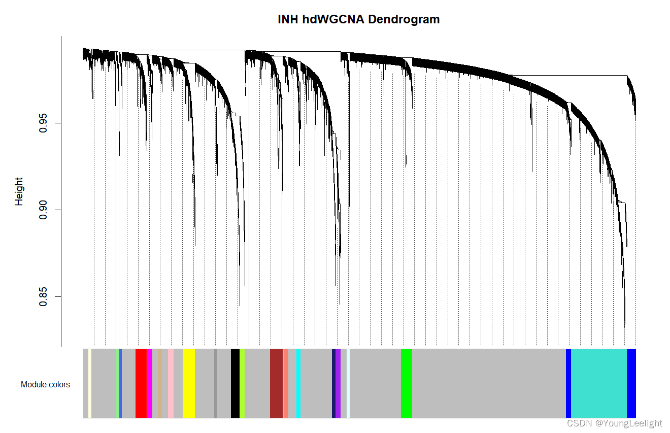

Optional: inspect the topoligcal overlap matrix (TOM)
hdWGCNA represents the co-expression network as a topoligcal overlap matrix (TOM). This is a square matrix of genes by genes, where each value is the topoligcal overlap between the genes. The TOM is written to the disk when running ConstructNetwork, and we can load it into R using the GetTOM function. Advanced users may wish to inspect the TOM for custom downstream analyses.
TOM <- GetTOM(seurat_obj)Module Eigengenes and Connectivity
In this section we will cover how to compute module eigengenes in single cells, and how to compute the eigengene-based connectivity for each gene.
Compute harmonized module eigengenes
Module Eigengenes (MEs) are a commonly used metric to summarize the gene expression profile of an entire co-expression module. Briefly, module eigengenes are computed by performing principal component analysis (PCA) on the subset of the gene expression matrix comprising each module. The first PC of each of these PCA matrices are the MEs.
Dimensionality reduction techniques are a very hot topic in single-cell genomics. It is well known that technical artifacts can muddy the analysis of single-cell datasets, and over the years there have been many methods that aim to reduce the effects of these artifacts. Therefore it stands to reason that MEs would be subject to these technical artifacts as well, and hdWGCNA seeks to alleviate these effects.
hdWGCNA includes a function ModuleEigengenes to compute module eigengenes in single cells. Additionally, we allow the user to apply Harmony batch correction to the MEs, yielding harmonized module eigengenes (hMEs). The following code performs the module eigengene computation harmonizing by the Sample of origin using the group.by.vars parameter.
# need to run ScaleData first or else harmony throws an error:
seurat_obj <- ScaleData(seurat_obj, features=VariableFeatures(seurat_obj))

# compute all MEs in the full single-cell dataset
seurat_obj <- ModuleEigengenes(
 seurat_obj,
 group.by.vars="Sample"
)
The ME matrices are stored as a matrix where each row is a cell and each column is a module. This matrix can be extracted from the Seurat object using the GetMEs function, which retrieves the hMEs by default.

> dim(seurat_obj)
[1] 36601 36671
# harmonized module eigengenes:
hMEs <- GetMEs(seurat_obj)

# module eigengenes:
MEs <- GetMEs(seurat_obj, harmonized=FALSE)
Compute module connectivity
In co-expression network analysis, we often want to focus on the “hub genes”, those which are highly connected within each module. Therefore we wish to determine the eigengene-based connectivity, also known as kME, of each gene. hdWGCNA includes the ModuleConnectivity to compute the kME values in the full single-cell dataset, rather than the metacell dataset. This function essentially computes pairwise correlations between genes and module eigengenes. kME can be computed for all cells in the dataset, but we recommend computing kME in the cell type or group that was previously used to run ConstructNetwork.
# compute eigengene-based connectivity (kME):
seurat_obj <- ModuleConnectivity(
  seurat_obj,
  group.by = 'cell_type', group_name = 'INH'
)
For convenience, we re-name the hdWGCNA modules to indicate that they are from the inhibitory neuron group. More information about renaming modules can be found in the module customization tutorial.
# rename the modules
seurat_obj <- ResetModuleNames(
seurat_obj,
new_name = "INH-M"
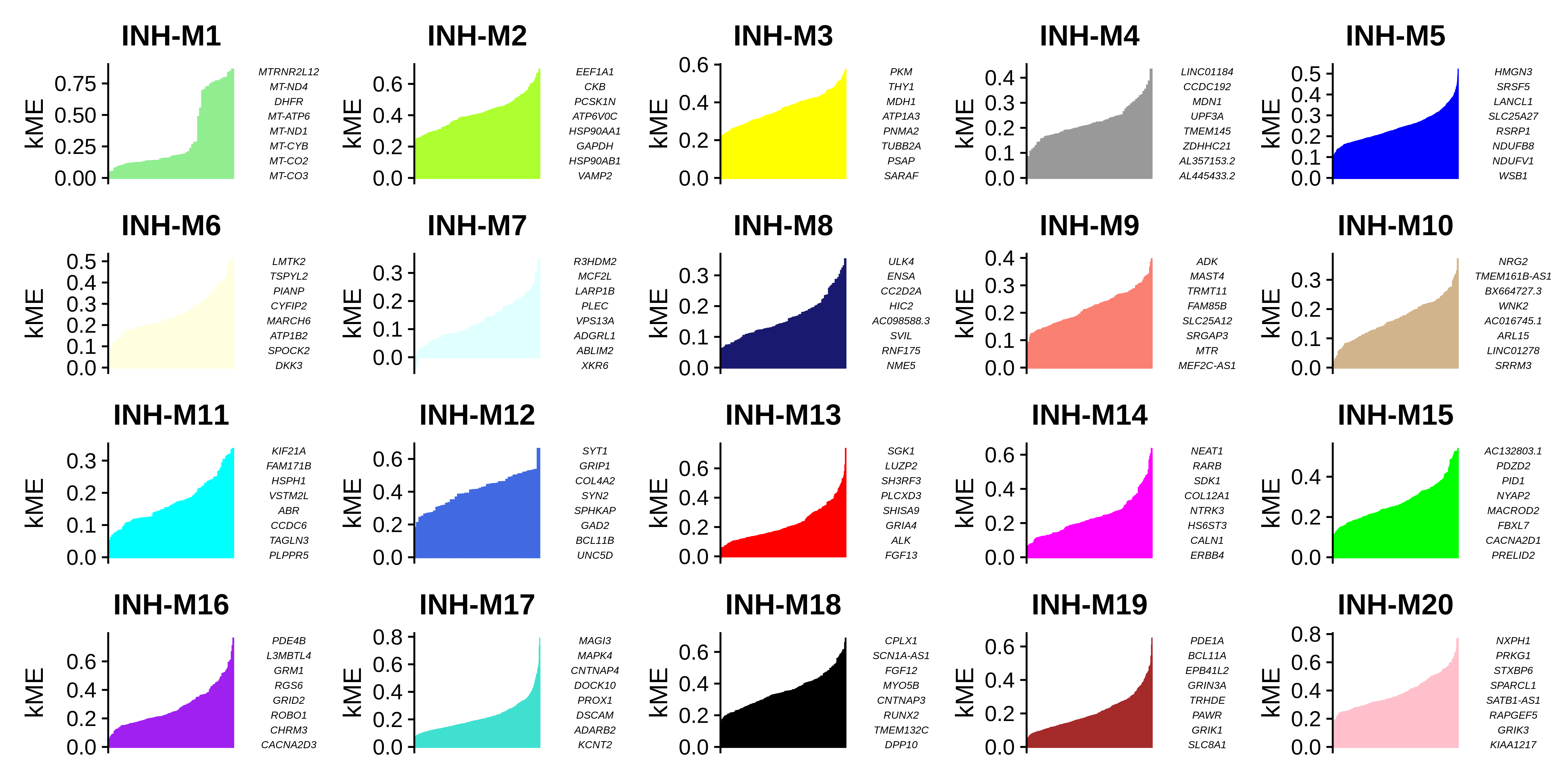
)We can visualize the genes in each module ranked by kME using the PlotKMEs function.
# plot genes ranked by kME for each module
p <- PlotKMEs(seurat_obj, ncol=5)

p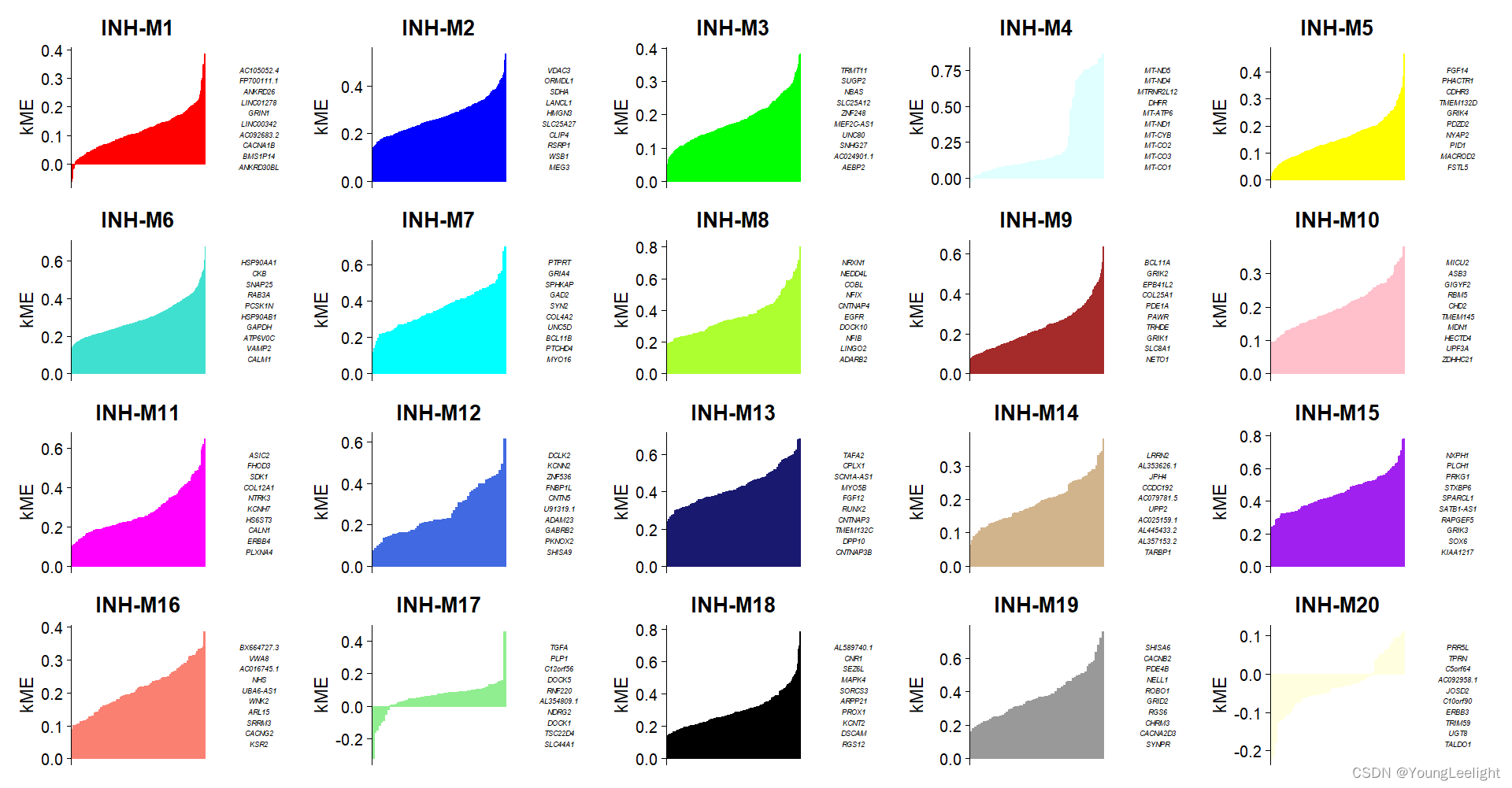
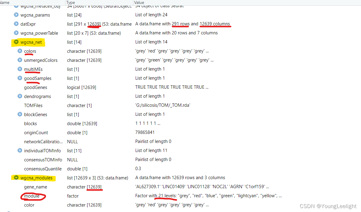
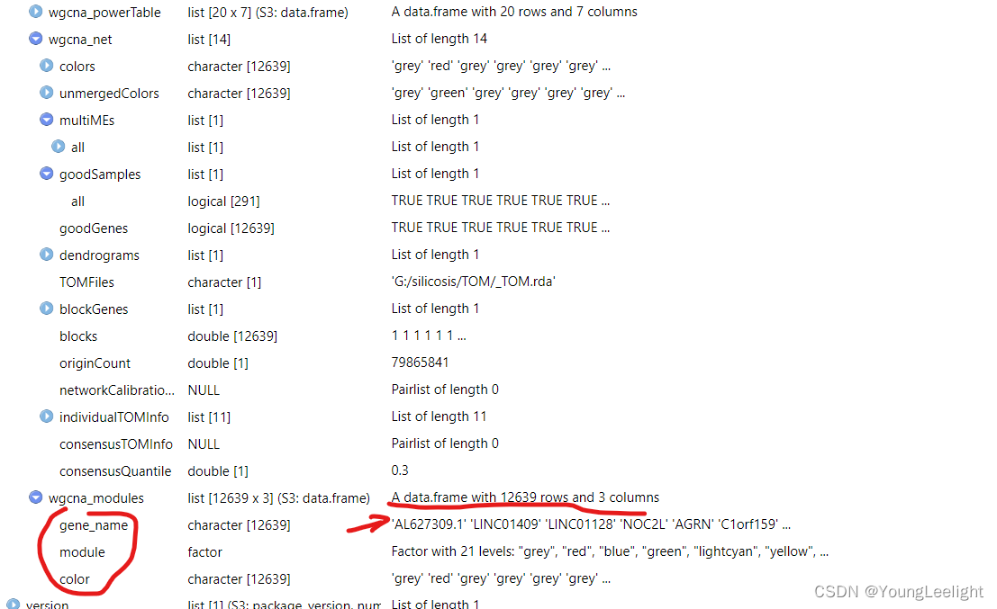
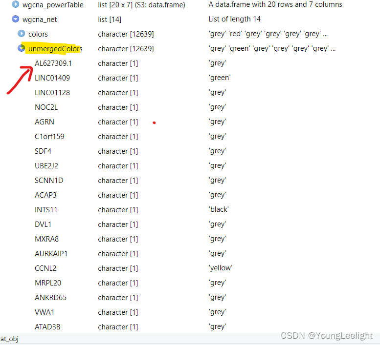
Getting the module assignment table
hdWGCNA allows for easy access of the module assignment table using the GetModules function. This table consists of three columns: gene_name stores the gene’s symbol or ID, module stores the gene’s module assignment, and color stores a color mapping for each module, which is used in many downstream plotting steps. If ModuleConnectivity has been called on this hdWGCNA experiment, this table will have additional columns for the kME of each module.
# get the module assignment table:
modules <- GetModules(seurat_obj)

# show the first 6 columns:
head(modules[,1:6])
Output
A table of the top N hub genes sorted by kME can be extracted using the GetHubGenes function.
# get hub genes
hub_df <- GetHubGenes(seurat_obj, n_hubs = 10)

head(hub_df)
Output
This wraps up the critical analysis steps for hdWGCNA, so remember to save your output.
saveRDS(seurat_obj, file='hdWGCNA_object.rds')Compute hub gene signature scores
Gene scoring analysis is a popular method in single-cell transcriptomics for computing a score for the overall signature of a set of genes. Seurat implements their own gene scoring technique using the AddModuleScore function, but there are also alternative approaches such as UCell. hdWGCNA includes the function ModuleExprScore to compute gene scores for a give number of genes for each module, using either the Seurat or UCell algorithm. Gene scoring is an alternative way of summarizing the expression of a module from computing the module eigengene.
# compute gene scoring for the top 25 hub genes by kME for each module
# with Seurat method
seurat_obj <- ModuleExprScore(
  seurat_obj,
  n_genes = 25,
  method='Seurat'
)

# compute gene scoring for the top 25 hub genes by kME for each module
# with UCell method
library(UCell)
seurat_obj <- ModuleExprScore(
  seurat_obj,
  n_genes = 25,
  method='UCell'
)
Basic Visualization
Here we showcase some of the basic visualization capabilities of hdWGCNA, and we demonstrate how to use some of Seurat’s built-in plotting tools to visualize our hdWGCNA results. Note that we have a separate tutorial for visualization of the hdWGCNA networks.
Module Feature Plots
FeaturePlot is a commonly used Seurat visualization to show a feature of interest directly on the dimensionality reduction. hdWGCNA includes the ModuleFeaturePlot function to consruct FeaturePlots for each co-expression module colored by each module’s uniquely assigned color.
# make a featureplot of hMEs for each module
plot_list <- ModuleFeaturePlot(
  seurat_obj,
  features='hMEs', # plot the hMEs
  order=TRUE # order so the points with highest hMEs are on top
)

# stitch together with patchwork
wrap_plots(plot_list, ncol=6)
转存失败重新上传取消
We can also plot the hub gene signature score using the same function:
# make a featureplot of hub scores for each module
plot_list <- ModuleFeaturePlot(
  seurat_obj,
  features='scores', # plot the hub gene scores
  order='shuffle' # order so cells are shuffled
  ucell = TRUE # depending on Seurat vs UCell for gene scoring
)

# stitch together with patchwork
wrap_plots(plot_list, ncol=6)
转存失败重新上传取消
Module Correlations
hdWGCNA includes the ModuleCorrelogram function to visualize the correlation between each module based on their hMEs, MEs, or hub gene scores using the R package corrplot.
# plot module correlagram
ModuleCorrelogram(seurat_obj)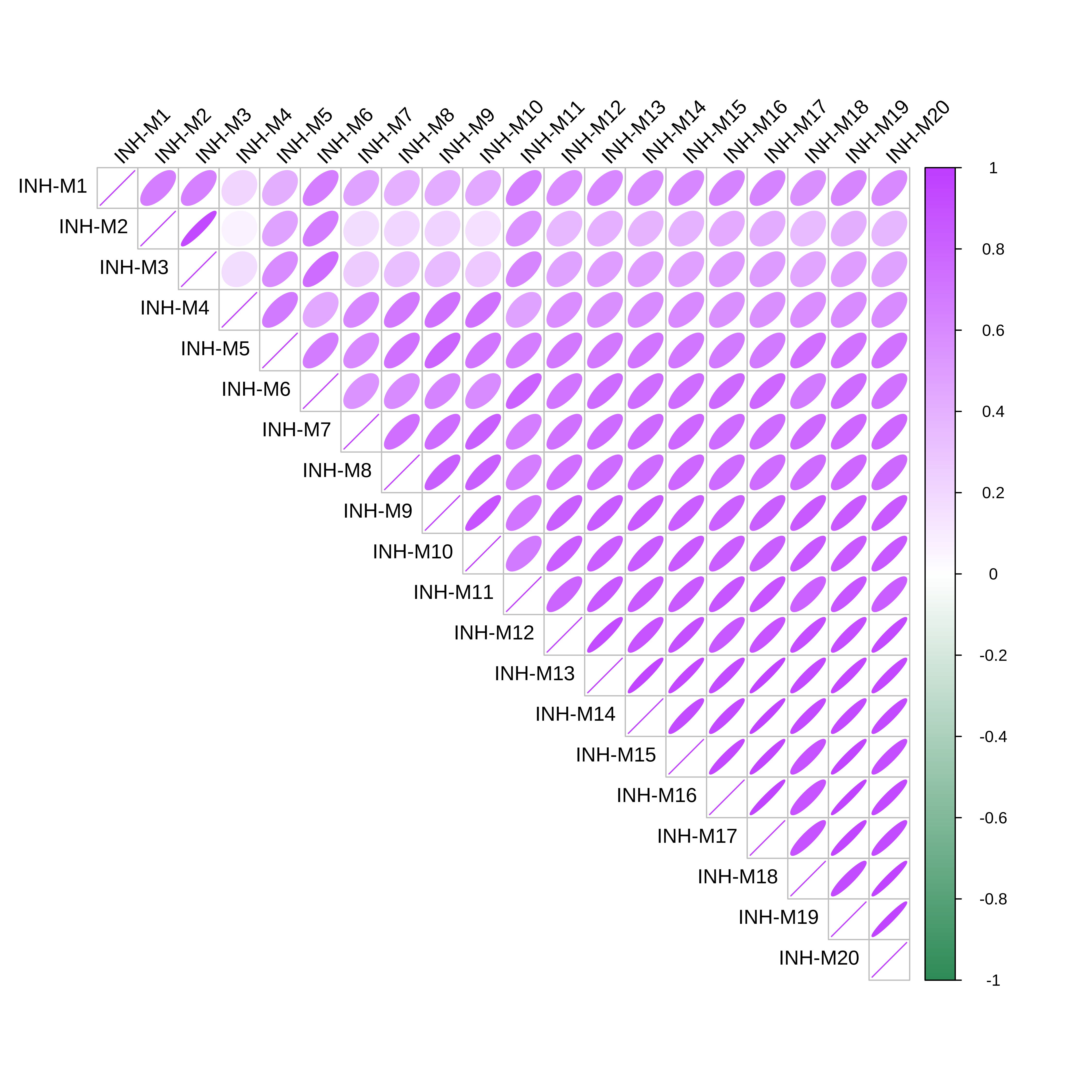
Seurat plotting functions
The base Seurat plotting functions are also great for visualizing hdWGCNA outputs. Here we demonstrate plotting hMEs using DotPlot and VlnPlot. The key to using Seurat’s plotting functions to visualize the hdWGCNA data is to add it into the Seurat object’s @meta.data slot:
# get hMEs from seurat object
MEs <- GetMEs(seurat_obj, harmonized=TRUE)
mods <- colnames(MEs); mods <- mods[mods != 'grey']

# add hMEs to Seurat meta-data:
seurat_obj@meta.data <- cbind(seurat_obj@meta.data, MEs)
Now we can easily use Seurat’s DotPlot function:
# plot with Seurat's DotPlot function
p <- DotPlot(seurat_obj, features=mods, group.by = 'cell_type')

# flip the x/y axes, rotate the axis labels, and change color scheme:
p <- p +
  coord_flip() +
  RotatedAxis() +
  scale_color_gradient2(high='red', mid='grey95', low='blue')

# plot output
p
正在上传…重新上传取消
Here is another example where we use Seurat’s VlnPlot function:
# Plot INH-M4 hME using Seurat VlnPlot function
p <- VlnPlot(
  seurat_obj,
  features = 'INH-M12',
  group.by = 'cell_type',
  pt.size = 0 # don't show actual data points
)

# add box-and-whisker plots on top:
p <- p + geom_boxplot(width=.25, fill='white')

# change axis labels and remove legend:
p <- p + xlab('') + ylab('hME') + NoLegend()

# plot output
p
正在上传…重新上传取消
Next steps
In this tutorial we went over the core functions for performing co-expression network analysis in single-cell transcriptomics data. We encourage you to explore our other tutorials for downstream analysis of these hdWGCNA results.


 1026
1026

 被折叠的 条评论
为什么被折叠?
被折叠的 条评论
为什么被折叠?
 到【灌水乐园】发言


