单细胞三大R包之monocle

0.准备R包和数据

library(monocle)
library(scRNAseq)
library(dplyr)

使用scRNAseq里面的示例数据fluidigm。这个示例数据本身是一个对象，我们又需要从中提取出来自己想要的组成部分，然后组成新的对象。
曾经fluidigm是一个可以用data提取的数据，后来包更新了，只能用下面的函数来调用咯

fluidigm = ReprocessedFluidigmData()
# Set assay to RSEM estimated counts
assay(fluidigm)  <-  assays(fluidigm)$rsem_counts
ct <- floor(assays(fluidigm)$rsem_counts)
ct[1:4,1:4]

##          SRR1275356 SRR1274090 SRR1275251 SRR1275287
## A1BG              0          0          0          0
## A1BG-AS1          0          0          0          0
## A1CF              0          0          0          0
## A2M               0          0          0         33

dim(ct) #count矩阵，行是基因，列是细胞

## [1] 26255   130

可以看到这里是有130个细胞，两万六千多个基因。

sample_ann <- as.data.frame(colData(fluidigm))
table(sample_ann$Biological_Condition)

## 
##   GW16   GW21 GW21+3    NPC 
##     52     16     32     30

细胞注释数据里提供了Biological Condition，后续的分析是以它为中心来分析的。

1.构建CellDataSet对象

gene_ann <- data.frame(
  gene_short_name = row.names(ct),
  row.names = row.names(ct)
)

pd <- new("AnnotatedDataFrame",
          data=sample_ann)
fd <- new("AnnotatedDataFrame",
          data=gene_ann)

cds <- newCellDataSet(
  ct,
  phenoData = pd,
  featureData =fd,
  expressionFamily = negbinomial.size(),
  lowerDetectionLimit=1)
class(cds)

## [1] "CellDataSet"
## attr(,"package")
## [1] "monocle"

## 为了电脑的健康，我这里选择小数据集。
cds <- estimateSizeFactors(cds)
cds <- estimateDispersions(cds)

2.质控

过滤前是26255 features, 130 samples,筛掉在5个以下细胞中表达的基因。这个标准是非常低的咯。

dim(cds)

## Features  Samples 
##    26255      130

cds <- detectGenes(cds, min_expr = 0.1)

head(fData(cds))

##          gene_short_name num_cells_expressed
## A1BG                A1BG                  10
## A1BG-AS1        A1BG-AS1                   2
## A1CF                A1CF                   1
## A2M                  A2M                  21
## A2M-AS1          A2M-AS1                   3
## A2ML1              A2ML1                   9

k = fData(cds)$num_cells_expressed>=5;table(k)

## k
## FALSE  TRUE 
## 12870 13385

cds <- cds[k,]
cds

## CellDataSet (storageMode: environment)
## assayData: 13385 features, 130 samples 
##   element names: exprs 
## protocolData: none
## phenoData
##   sampleNames: SRR1275356 SRR1274090 ... SRR1275261 (130 total)
##   varLabels: NREADS NALIGNED ... num_genes_expressed (30 total)
##   varMetadata: labelDescription
## featureData
##   featureNames: A1BG A2M ... ZZZ3 (13385 total)
##   fvarLabels: gene_short_name num_cells_expressed
##   fvarMetadata: labelDescription
## experimentData: use 'experimentData(object)'
## Annotation:

dim(cds)

## Features  Samples 
##    13385      130

过滤基因后是：13385 features, 130 samples，很低的标准也过滤掉了一半的基因。

fivenum(pData(cds)$NREADS)

## [1]    91616   232899   892209  8130850 14477100

fivenum(pData(cds)$num_genes_expressed)

## [1] 1418.0 2961.0 3841.5 5381.0 8221.0

NREADS展示了每个细胞中总共多少条reads，num_genes_expressed展示了每个细胞中有多少个基因表达量不为0。可以根据这两个指标设置阈值去过滤细胞。在这里不需要过滤。

3.聚类

筛选平均表达量 > 0.1的基因用于聚类

disp_table <- dispersionTable(cds)
unsup_clustering_genes <- subset(disp_table, mean_expression >= 0.1)

cds <- setOrderingFilter(cds, unsup_clustering_genes$gene_id)

碎石图，降维和细胞聚类

plot_pc_variance_explained(cds, 
                           return_all = F,
                           max_components = 20)

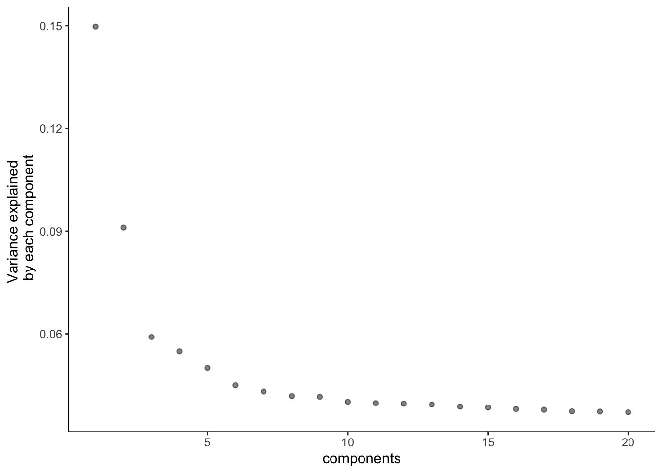
# 其中 num_dim 参数选择基于上面的PCA图
cds <- reduceDimension(cds, 
                       max_components = 2, 
                       num_dim = 6,
                       reduction_method = 'tSNE', verbose = T)
cds <- clusterCells(cds, num_clusters = 4)

## Distance cutoff calculated to 0.5395435

plot_cell_clusters(cds, 1, 2,
                   color = "Biological_Condition")

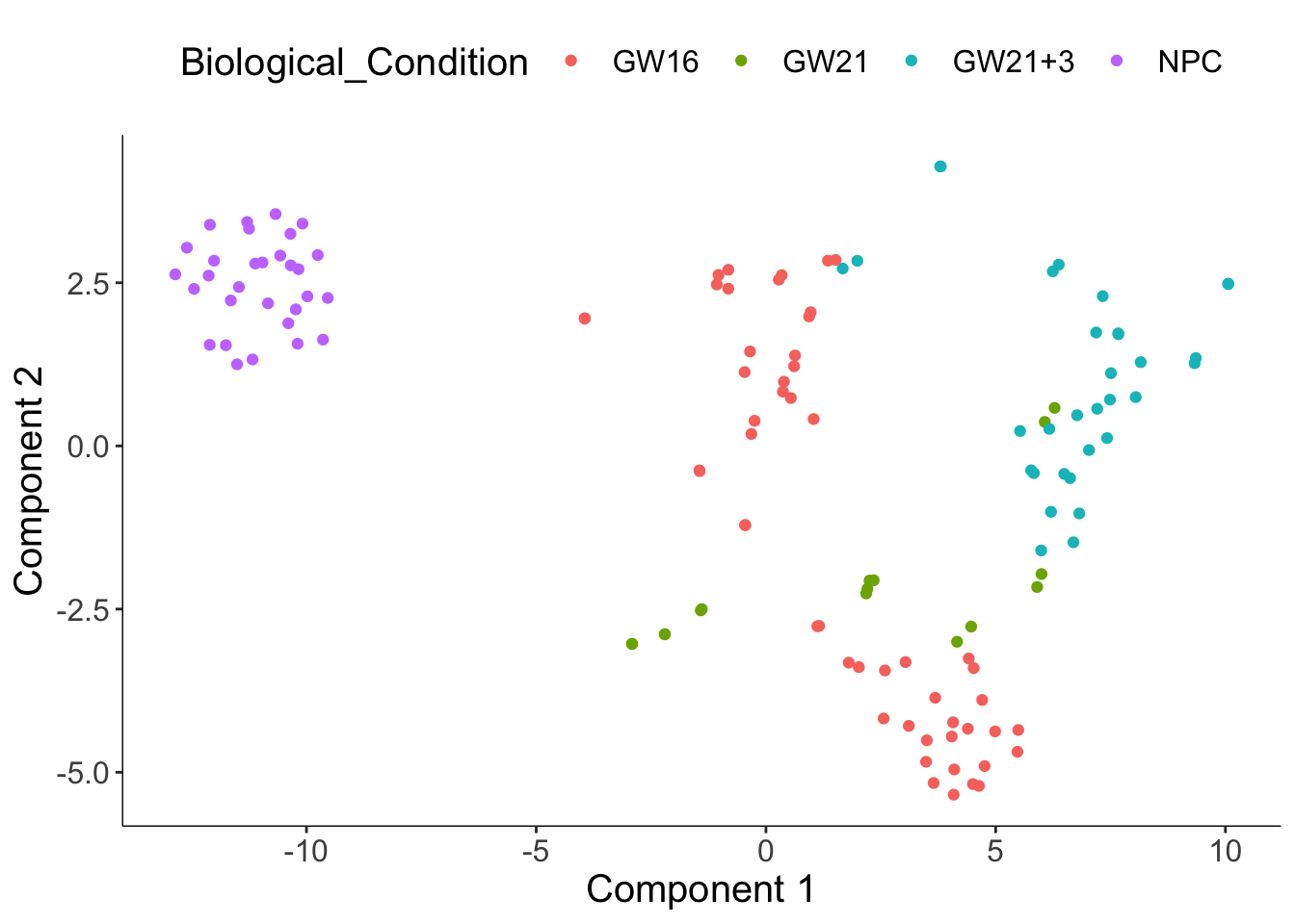
发现聚类结果与Biological Condition高度吻合。如果不指定颜色的话，是按照聚出来的细胞簇来分配颜色。

如果有需要去除的干扰因素，可以使用reduceDimension里的 residualModelFormulaStr参数，去除干扰因素再聚类。

4.差异分析

找差异基因的过程给做成函数咯。

diff_test_res <- differentialGeneTest(cds,
                                      fullModelFormulaStr = "~Biological_Condition")
# Select genes that are significant at an FDR < 10%
sig_genes <- subset(diff_test_res, qval < 0.1)
dim(sig_genes)

## [1] 6427    7

head(sig_genes[,c("gene_short_name", "pval", "qval")] )

##       gene_short_name         pval         qval
## A1BG             A1BG 6.759792e-04 2.362397e-03
## A2M               A2M 5.659195e-08 5.852474e-07
## AACS             AACS 3.329596e-03 9.677356e-03
## AADAT           AADAT 1.403810e-02 3.422585e-02
## AAGAB           AAGAB 1.717061e-07 1.540937e-06
## AAMP             AAMP 8.820175e-05 3.849301e-04

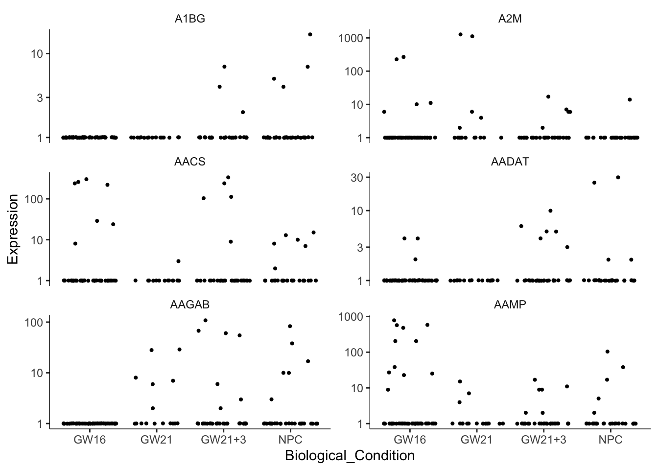
还可以很方便的指定基因画表达量散点图。横坐标没有意义，每个点是一个细胞。

cg = head(sig_genes$gene_short_name)
plot_genes_jitter(cds[cg,],
                  grouping = "Biological_Condition", 
                  ncol= 2)

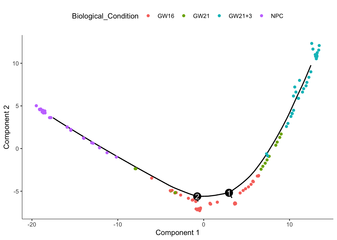
5.推断发育轨迹

挑选差异显著的基因（q<0.01）做降维，给细胞排序

ordering_genes <- row.names (subset(diff_test_res, qval < 0.01));length(ordering_genes)

## [1] 4617

cds <- setOrderingFilter(cds, ordering_genes)
cds <- reduceDimension(cds, max_components = 2,
                       method = 'DDRTree')
# 细胞排序
cds <- orderCells(cds)
# 可视化
plot_cell_trajectory(cds, color_by = "Biological_Condition")

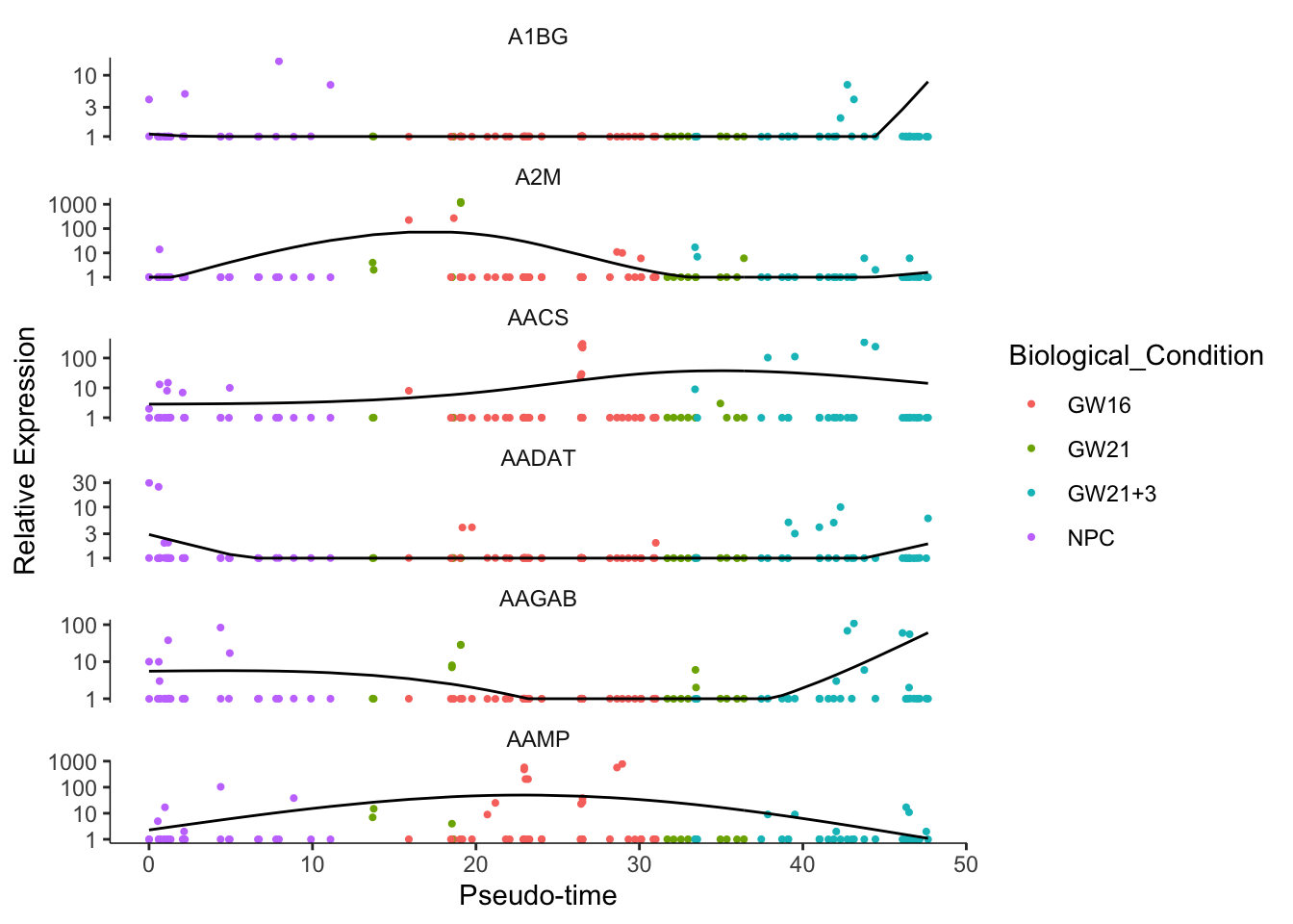
# 展现marker基因
plot_genes_in_pseudotime(cds[cg,],
                         color_by = "Biological_Condition")