


💥💥💞💞欢迎来到本博客❤️❤️💥💥
🏆博主优势:🌞🌞🌞博客内容尽量做到思维缜密,逻辑清晰,为了方便读者。
⛳️座右铭:行百里者,半于九十。
📋📋📋本文目录如下:🎁🎁🎁
目录
💥1 概述
KEWLS和KEWLS-KF是一种新的状态估计方法,它们采用低维线性卡尔曼滤波器将单个传感器的测量外推/预测到单个估计瞬间。这些方法主要用于WLS多点定位方法,可以提高定位的精度和鲁棒性。
KEWLS和KEWLS-KF方法的核心是卡尔曼滤波器,它可以通过对系统动态模型和测量模型进行有效的状态估计。通过将单个传感器的测量外推/预测到单个估计瞬间,KEWLS和KEWLS-KF可以有效地处理传感器测量中的噪声和不确定性,从而提高定位的精度和鲁棒性。
与传统的WLS多点定位方法相比,KEWLS和KEWLS-KF方法具有更好的性能,尤其是在复杂环境和噪声干扰下。这些方法可以应用于各种领域,如室内定位、车辆定位和机器人定位等,为实时定位和导航提供了新的可能性。因此,KEWLS和KEWLS-KF方法在状态估计领域具有重要的研究意义和实际应用前景。
摘要
本文代码运行了一个变量定位模拟,其中四个独立的传感器测量它们与动态目标的各自距离。然而,这些测量是按顺序接收的。这些测量之间的时间差是恒定的,并被称为测量间延迟(IML)。这自然会导致定位估计的误差。
模拟了可变位置服务,以确定IML的影响,并提出了用于顺序异步定位的方法(KEWLS/KKF)。
该模型作为批量模拟运行,其中每个传感器提供其嘈杂的测量估计,并采用各种位置技术来提供最终的估计。
关键变量
首先,该模型被构建为跟踪一个对象在直线或圆形路径上的运动。可以调整变量以改变轨迹、动力学、噪声水平、速度等。
d_t = IML(秒)
r_z = 单个传感器测量噪声标准差
q = KEWLS卡尔曼外推过程Q的标准差/预测D
qt = CV模型中过程Q加速度的标准差
ang = 0.2;%圆形路径的角度
其他模拟设置变量
bl = 传感器之间的基线距离(米)
Lim = 旅行限制的基线倍增器
xV = 目标x轴速度(米/秒)
yV = 目标y轴速度(米/秒)
move_noise = 目标移动噪声标准差(米)
s_pos = 目标起始位置
delay = 1;%将d_t延迟测量(如果不需要延迟,则设为0)
模型
该模型生成了与各种定位方法的准确性和运行时间相关的各种图表。
结构
可以选择一个变量通过一系列循环进行变化,在这些循环中,所选择的变量将在“Var”的下一个数组值中循环,可以使用lin/log或手动设置来改变“Var”:
Var = linspace(0.001,0.1,No_loops); %从第二个值开始
Var = logspace(-2,3,No_loops); %从第二个值开始
Var = [0.001,.002,.003,.004,.005,.006,.007,.008,.009,...
.01,.02,.03,.04,.05,.06,.07,.08,.09,...
.1,.2,.3,.4,.5,.6,.7,.8,.9,1];
一定要在这里更改数值!
r_z = Var(loop);
ChangingVar = 'r_z';
设置^^这将允许在最后进行自动标记
No_loops = 28;%变量循环次数(如果手动设置了Var的值,应该等于length(Var))
通过每个变量,模拟将重复“No_it”次,以计算平均值。
No_it = 100;%迭代次数
鉴于tic/toc函数在10毫秒以下的不准确性,可以进一步重复“No_times”次,以给出各个定位方法的可用时间估计。
No_times = 1;%重复进行tic/toc函数的次数
建议将其保留为1,除非需要专门测量计算时间。
过程
模型最初运行并使用“DelayedLaterationFunc”或“DelayedLaterationFunc_circ”(如果ang~=0)收集完整的嘈杂测量数据。
然后,这些数据被分别输入到各种定位方法中,以提供它们各自的估计。
对于每个变量值的每次迭代,都会重复这一过程,利用平均值来确定RMSE、路径和一般跟踪性能。
KEWLS和KKF
这些是采用低维线性卡尔曼滤波器将单个传感器测量外推/预测到单个估计瞬间,用于WLS多点定位方法的新方法。
结果
在“Results”目录下已经给出了多种场景的结果。
📚2 运行结果


主函数部分代码:
clear all
clc
%%run variable loop
%%/
%here we will change a variable and run it through the 'loop'
No_loops = 28; %number of variable loops
No_it = 100; %number of iterations
No_times = 1; %number of times a process is repeated for tic/toc func
%loop storage
LS_RMSE = zeros(1,No_loops); %classic least squares
UKF_RMSE = zeros(1,No_loops); %classic Unscented Kalman filter
KEWLS_RMSE = zeros(1,No_loops); %proposed = Sequential extrapolation / batch estimation
KKF_RMSE = zeros(1,No_loops); %proposed but with an additional KF
SUKF_RMSE = zeros(1,No_loops); %sequential Unscented Kalman filter
LS_mean = cell(1,No_loops); %classic least squares
UKF_mean = cell(1,No_loops); %classic Unscented Kalman filter
KEWLS_mean = cell(1,No_loops); %proposed = Sequential extrapolation / batch estimation
KKF_mean = cell(1,No_loops); %proposed but with an additional KF
SUKF_mean = cell(1,No_loops); %sequential Unscented Kalman filter
LS_t = zeros(1,No_loops);
UKF_t = zeros(1,No_loops);
KEWLS_t = zeros(1,No_loops);
KKF_t= zeros(1,No_loops);
SUKF_t = zeros(1,No_loops);
%%// VARIABLES
bl = 10; %baseline
Lim = 1; %basline multiplier for travel limits
xV = 1;
yV = 1;
move_noise = 0; %Movement noise StD
s_pos = [0 ; 0]; %target start Position
delay = 1; % LEAVE AS 1 to delay the measurements by d_t or not
R = RRLH2D_positions(bl); %generate pos of rx's
.....
%% storage in cells for each variable iteration
posX = cell(1,250);
posY = cell(1,250);
M_posX = cell(1,250);
M_posY = cell(1,250);
Measurments = cell(1,250); % noisy measurments
True_distances = cell(1,250); % actual distances
True_dis_atEstPos = cell(1,250); % actual distances at the estimation point
%% Least squares and two step least squares
LS_estX = cell(1,250);
LS_estY = cell(1,250);
LS_Errors = cell(1,250);
LS_time = zeros(1,100);
%% Classic Unscented Kalman filter
UKF_estX = cell(1,250);
UKF_estY = cell(1,250);
UKF_Errors = cell(1,250);
UKF_time = zeros(1,100);
%% KEWLS
KEWLS_estX = cell(1,250);
KEWLS_estY = cell(1,250);
KEWLS_Errors = cell(1,250);
KEWLS_time = zeros(1,100);
%% KEWLS-KF (KKF)
KKF_estX = cell(1,250);
KKF_estY = cell(1,250);
KKF_Errors = cell(1,250);
KKF_time = zeros(1,100);
%% SUKF solution
SUKF_estX = cell(1,250);
SUKF_estY = cell(1,250);
SUKF_Errors = cell(1,250);
SUKF_time = zeros(1,100);
%%/// RUN ITERATIONS //
%% ITERATIONS
%% generate a circular path
C_path = 0;
if ang ~= 0
%distance per simulation time interval = time interval to mainatin 1m/s
Radius = 1/ang;
No_steps = (2*pi*Radius)/0.0001; %circumfrence distance/simulation time
C_path = circle_move(Radius,bl,No_steps);
end
%run through iterations
for it = 1:No_it
%Run the simulation to collect measurment data
if ang == 0
[True_est_pos, measurment_pos, measurments, true_distances, true_dis_atEstPos] =...
DelayedLaterationFunc_Str(R, delay, bl, Lim, xV, yV, d_t, s_pos, r_z, move_noise);
else
[True_est_pos, measurment_pos, measurments, true_distances, true_dis_atEstPos] =...
DelayedLaterationFunc_circ(R, delay, bl, Lim, xV, yV, d_t, s_pos, C_path, r_z, move_noise);
end
% store data
%legendCell{it} = append(num2str(d_t),'s'); %convert d_t to string for legend
posX{it} = True_est_pos(1,:);
posY{it} = True_est_pos(2,:);
M_posX{it} = measurment_pos(1,:);
M_posY{it} = measurment_pos(2,:);
Measurments{it} = measurments;
True_distances{it} = true_distances;
True_dis_atEstPos{it} = true_dis_atEstPos;
%% perform standard LS on the measurments - (currently TS is turned off for fair timing)
可视化部分代码:
%% RMSE error %%%%%%%%%%%%%%%%%%%%%%%%%%%%%%%%%%%%%%%%%%%%%%%%%%%%%%%%%%%%%
figure(1)
hold on
plot(Var,LS_RMSE,'-.')
plot(Var,UKF_RMSE,'-.')
plot(Var,SUKF_RMSE, '--')
plot(Var,KEWLS_RMSE)
plot(Var,KKF_RMSE)
legend('LS','UKF','SUKF','KEWLS', 'K-KF')
ylabel('RMSE/m')
xlabel(label)
T = append('System RMSE with varied ', ChangingVar);
title(T)
hold off
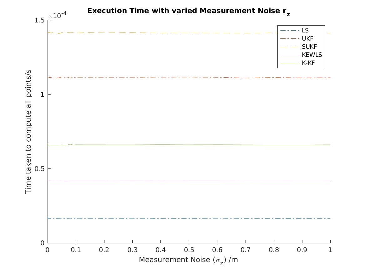
%% execution time %%%%%%%%%%%%%%%%%%%%%%%%%%%%%%%%%%%%%%%%%%%%%%%%%%%%%%%%%
figure(2)
hold on
plot(Var,LS_t,'-.')
plot(Var,UKF_t,'-.')
plot(Var,SUKF_t, '--')
plot(Var,KEWLS_t)
plot(Var,KKF_t)
legend('LS','UKF','SUKF','KEWLS', 'K-KF')
ylabel('Time taken to compute all points/s')
xlabel(label)
T = append('Execution Time with varied ', ChangingVar);
title(T)
hold off
%% Last Loop avererage errors %%%%%%%%%%%%%%%%%%%%%%%%%%%%%%%%%%%%%%%%%%%%%
figure(3)
hold on
plot(LS_me,'-.')
plot(UKF_me,'-.')
plot(SUKF_me,'--')
plot(KEWLS_me)
plot(KKF_me)
legend('LS','UKF','SUKF','KEWLS','K-KF')
xlabel('Iteration')
T = append('Average Error with varied ', ChangingVar);
title(T)
hold off
%% Last Loop, last iteration, errors %%%%%%%%%%%%%%%%%%%%%%%%%%%%%%%%%%%%%%
figure(4)
hold on
for i = 1:1%it
plot(LS_Errors{i}(1,3:end),'-.')
plot(UKF_Errors{i}(1,3:end),'-.')
plot(SUKF_Errors{i}(1,3:end),'--')
plot(KEWLS_Errors{i})
plot(KKF_Errors{i})
end
legend('LS','UKF','SUKF','KEWLS','K-KF')
ylabel('Error /m')
xlabel('Iteration')
T = append('Last iteration error with varied ', ChangingVar);
title(T)
hold off
%% Path Plot & Estimate points %%%%%%%%%%%%%%%%%%%%%%%%%%%%%%%%%%%%%%%%%%%%
figure(5)
hold on
%plot user positions
for i = 1:1%iteration-1
plot(posX{i},posY{i},'+')
end
%plot LS estimates
for i = 1:1%iteration-1
plot(LS_estX{i},LS_estY{i},'*')
end
%plot proposed estimates
for i = 1:1%iteration-1
plot(KEWLS_estX{i},KEWLS_estY{i}, 'p')
end
%plot UKF estimates
for i = 1:1%iteration-1
plot(UKF_estX{i},UKF_estY{i}, 'x')
end
%plot UKF estimates
for i = 1:1%iteration-1
plot(SUKF_estX{i},SUKF_estY{i}, 'o')
end
%plots lines between each estimate and position.
for i = 1:1%iteration-1
for j = 1:length(LS_estX{i})
x = [LS_estX{i}(j) , posX{i}(j)];
y = [LS_estY{i}(j) , posY{i}(j)];
plot(x,y,'--','LineWidth',2)
end
end
%plots lines between each estimate and position.
for i = 1:1%iteration-1
for j = 1:length(KEWLS_estX{i}(1,1:end-2))
x = [KEWLS_estX{i}(j) , posX{i}(j+2)];
y = [KEWLS_estY{i}(j) , posY{i}(j+2)];
plot(x,y,'LineWidth',2)
end
end
%plots lines between each estimate and position.
for i = 1:1%iteration-1
for j = 1:length(SUKF_estX{i})
x = [SUKF_estX{i}(j) , posX{i}(j)];
y = [SUKF_estY{i}(j) , posY{i}(j)];
plot(x,y,'-.','LineWidth',2)
end
end
%plots lines between each estimate and position.
for i = 1:1%iteration-1
for j = 1:length(UKF_estX{i})
x = [UKF_estX{i}(j) , posX{i}(j)];
y = [UKF_estY{i}(j) , posY{i}(j)];
plot(x,y,'-.','LineWidth',2)
end
end
axis equal
scatter(R(1,:),R(2,:),100,'^','LineWidth',2) %show the RRLHs
%legend(legendCell)
legend('UT position','LS est', 'KEWLS', 'UKF' , 'SUKF')
T = append('Path plot with varied ', ChangingVar);
title(T)
xlabel('X position /m')
ylabel('Y position /m)')
hold off
%% Path Plot
figure(6)
hold on
plot(posX{1},posY{1})
plot(LS_estX{1},LS_estY{1})
plot(UKF_estX{1},UKF_estY{1})
plot(SUKF_estX{1},SUKF_estY{1})
plot(KEWLS_estX{1},KEWLS_estY{1})
plot(KKF_estX{1},KKF_estY{1})
axis equal
scatter(R(1,:),R(2,:),100,'^','LineWidth',2) %show the RRLHs
legend('Target Position','LS','UKF','SUKF','KEWLS','K-KF')
T = append('Path plot with varied ', ChangingVar);
title(T)
xlabel('X position /m')
ylabel('Y position /m)')
hold off
figure(10)
loglog(Var,LS_RMSE,'-.')
hold on
loglog(Var,UKF_RMSE,'-.')
loglog(Var,SUKF_RMSE, '--')
loglog(Var,KEWLS_RMSE)
loglog(Var,KKF_RMSE)
legend('LS','UKF','SUKF','KEWLS','K-KF')
ylabel('RMSE/m')
xlabel(label)
T = append('System RMSE with varied ', ChangingVar);
title(T)
hold off
🎉3 参考文献
文章中一些内容引自网络,会注明出处或引用为参考文献,难免有未尽之处,如有不妥,请随时联系删除。
[1]陈鹏,钱徽,朱淼良.基于加权最小二乘的卡尔曼滤波算法[J].计算机科学, 2009.DOI:JournalArticle/5af37a83c095d718d80ccec5.
[2]张肖雄.基于卡尔曼滤波的系统状态和荷载识别方法研究[D].湖南大学,2019.
[3]陈鹏,钱徽,朱淼良.基于加权最小二乘的卡尔曼滤波算法[J].计算机科学, 2009(11):236-237+263.DOI:CNKI:SUN:JSJA.0.2009-11-059.


 1万+
1万+


 被折叠的 条评论
为什么被折叠?
被折叠的 条评论
为什么被折叠?
 到【灌水乐园】发言


