基于预测控制模型的自适应巡航控制仿真与机器人实现（Matlab代码实现）

     目录

💥1 概述

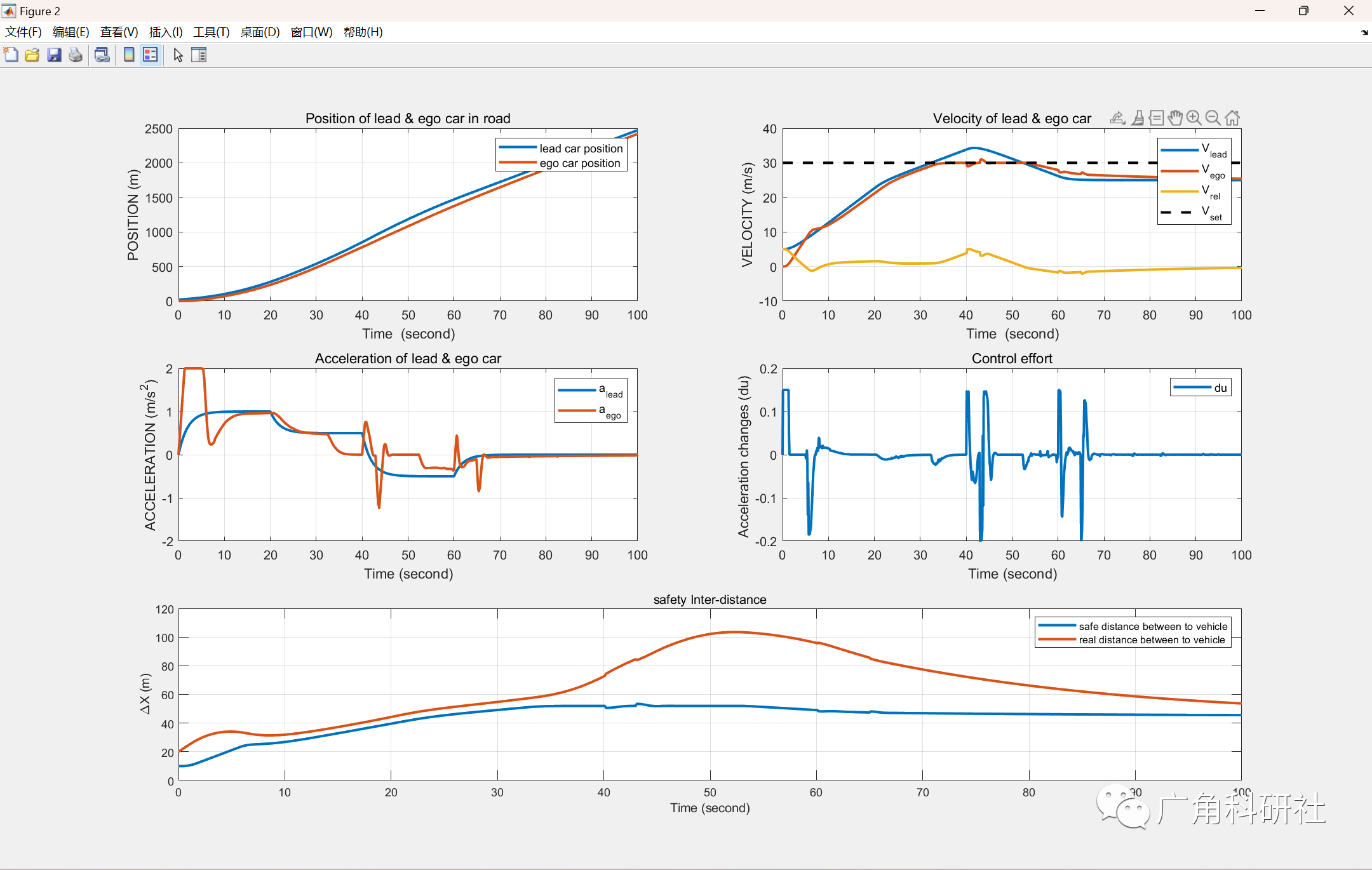
📚2 运行结果

🎉3 参考文献

👨‍💻4 Matlab代码

💥1 概述

自适应巡航控制技术为目前由于汽车保有量不断增长而带来的行车安全、驾驶舒适性及交通拥堵等问题提供了一条有效的解决途径，因此本文通过理论分析、仿真验证及实车实验对自适应巡航控制中的若干关键技术展开研究，以提高自适应巡航控制在不同工况下的应用能力。 ​

本研究为基于预测控制模型的自适应巡航控制仿真与机器人实现。

研究目的：

• 在两辆车之间已经达到了近乎精确的纵向模型
• 试图使控制响应接近可行性和真实条件。
• 满足防撞和保持安全距离，前车为主要目标，舒适性为次要目标。（控制应用于以下汽车）
• 在 MATLAB 上应用实现和仿真。

📚2 运行结果

主函数部分代码：

clear ;
close all;
clc

%
 Define the sample time, |Ts|, and simulation duration, |t|, in seconds.
t0 = 0;
Ts = 0.1;
Tf = 100;
t = t0:Ts:Tf;               
Nt = numel(t);
% Specify the initial position and velocity for the two vehicles.

%
x0_lead = 0;               %Initial position of lead car (m)
%v0_lead = 0;               %Initial velocity of lead car (m/s)

%
x0_ego = 0;                %Initial position of ego car (m)
%v0_ego = 0;                %Initial velocity of ego car (m/s)

%
 The safe distance between the lead car and the ego car is a function
% of the ego car velocity, $V_{ego}$:
%
% $$ D_{safe} = D_{default} + T_{gap}\times V_{ego} $$
%
% where $D_{default}$ is the standstill default spacing and $T_{gap}$ is
% the time gap between the vehicles. Specify values for $D_{default}$, in
% meters, and $T_{gap}$, in seconds.
t_gap = 1.4;
D_default = 10;

%
 Specify the driver-set velocity in m/s.
v_set = 30;

%
 Considering the physical limitations of the vehicle dynamics, the
% acceleration is constrained to the range  |[-3,2]| (m/s^2).
a_max = 2; da_max = 0.15;
a_min = -3; da_min = -0.2;

​
​
%
 the relationship between the actual acceleration and the desired 
% acceleration of the host vehicle satisfies the following conditions 
% 
%  $$ a(k+1) = (1-\frac{Ts}{\tau}) \times a(k) + \frac{Ts}{\tau} \times u(k)$$
%  
% where $ \tau $ is the time lag of the ACC system
tau = 0.3;

​
%
Np = 20 ;          % Prediction Horizon
%Nc = 20 ;          % Control Horizon

%
% Examples
%  In this section we want to try to specify the various parameters 
%   of the machine for different simulation

​
%
EX.1
% N = 5;
% Np = 20 ;          % Prediction Horizon
% Nc = 5 ;          % Control Horizon
% x0_ego  = 0;
% v0_ego  = 0;
% x0_lead = 50;
% v0_lead = 15;
% a_lead = 0.3*sin(2*pi*0.03*t);  % Acceleration of lead car is a disturbance for our plant;
% [lead_car_position , lead_car_velocity] = lead_car_simulation(x0_lead,v0_lead,a_lead,t,Ts ,tau);

%
 EX.2
N = 5;
Np = 20 ;          % Prediction Horizon
Nc = 15 ;          % Control Horizon
x0_ego  = 0;
v0_ego  = 0;
x0_lead = 20;
v0_lead = 5;
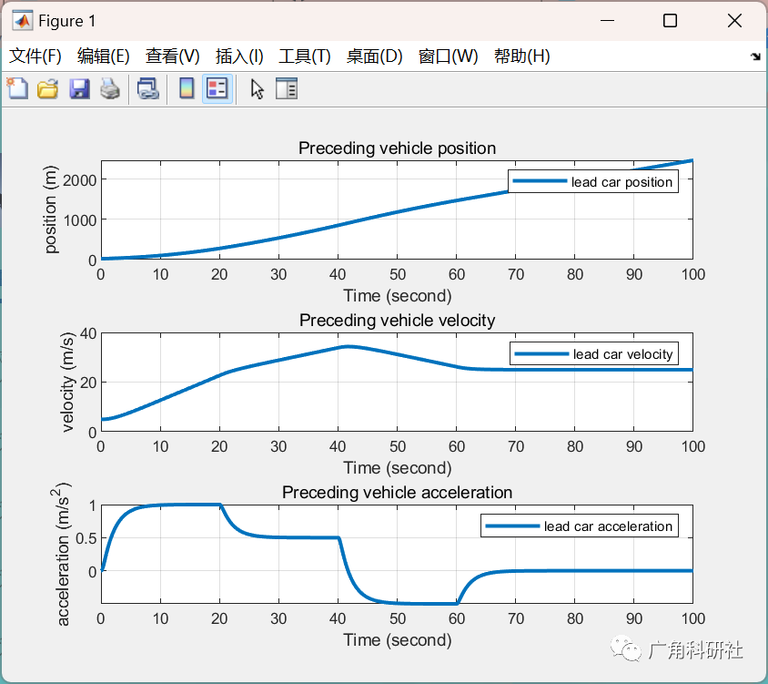
a_lead = [1*(1-exp(-0.5*t(1:floor(Nt/5)))) ,0.5+0.5*exp(-0.5*t(1:floor(Nt/5))) , -0.5+exp(-0.5*t(1:floor(Nt/5))) ,-0.5*exp(-0.5*t(1:floor(Nt/5))) , zeros(1,floor(Nt/5)+1)];  
[lead_car_position , lead_car_velocity] = lead_car_simulation(x0_lead,v0_lead,a_lead,t,Ts ,tau);

%
 % % EX.3
% Np = 20 ;          % Prediction Horizon
% Nc = 15 ;          % Control Horizon
% x0_ego  = 0;
% v0_ego  = 0;
% x0_lead = 1500;
% v0_lead = 0;
% a_lead = zeros(1,Nt) ;
% [lead_car_position , lead_car_velocity] = lead_car_simulation(x0_lead,v0_lead,a_lead,t,Ts ,tau);

%
% Car State Space Model
​
Am=[1   Ts   0.5*Ts^2
    0   1      Ts
    0   0     1-Ts/tau ];
​
Bm=[0 ; 0 ; Ts/tau];
​
Cm=[1   0  0
    0   1  0];
​
​
n = size(Am , 1) ;  % number of eigenvalues
q = size(Cm , 1) ;  % number of outputs
m = size(Bm , 2) ;  % number of inputs
​
​
[A , B , C] = AugemenFun(Am , Bm , Cm) ;
​
a = 0.5 ;
[Al , L0] = LagFun(N,a);
L = zeros( N , Nc ); 
L( : , 1) = L0 ; 
for i = 2:Nc
    L(:,i) = Al*L(: , i-1) ; 
end

🎉3 参考文献

[1]李朋,魏民祥,侯晓利.自适应巡航控制系统的建模与联合仿真[J].汽车工程,2012,34(07):622-626.

部分理论引用网络文献，若有侵权联系博主删除。