Plucker坐标与Plucker矩阵

Plucker坐标与Plucker矩阵

最近学习Plucker坐标相关内容时，发现找到的资料比较少，而且有许多相互矛盾之处，这里开坑一一记录一下。

几何定义

假设$\mathbf{x},\mathbf{y}$是直线上的点，直线的Plucker坐标表示为$\mathbf{L}:=(\mathbf{l},\mathbf{m})$，其中

• $\mathbf{l}=\mathbf{y}-\mathbf{x}$
• $\mathbf{m}=\mathbf{x}\times \mathbf{y}$
• $\frac{\Vert \mathbf{m}\Vert }{||\mathbf{l}||}$为原点到直线距离

plucker坐标有6个分量，但是受到约束 $\mathbf{m}\cdot \mathbf{l}=0$，以及齐次性，所以只有4个自由度。

注意，这一小节里的点都是3维的。下一小节用4维的齐次坐标了。

代数定义

假设$\mathbf{x}=(x_0,x_1,x_2,x_3{)}^T,\mathbf{y}=(y_0,y_1,y_2,y_3{)}^T$是齐次坐标，其中$x_0,y_0$是额外引入的尺度项（我实在没找到这一项该怎么叫，既然它的作用是表征尺度大小，在本文中就姑且叫它尺度项吧）。定义$l_{ij}=x_i{y}_j-x_j{y}_i$，那么不难验证在尺度项$x_0,y_0$都是1时，$\mathbf{l}=(l_{01},l_{02},l_{03}{)}^T$，$\mathbf{m}=(l_{23},l_{31},l_{12}{)}^T$

于是Plucker坐标可以表示为
$$\mathbf{L}=(l_{01},l_{02},l_{03},l_{23},l_{31},l_{12}{)}^T$$

注意,在这里，我们把下标0当成了尺度项，这会让两种定义的坐标顺序是对应的。但是有些文章里坐标的顺序甚至下标的顺序（31还是13）都不一样。但这不是很重要，因为实际运算里还是用$\mathbf{l},\mathbf{m},l_{ij}$这种定义明确的符号比较多

Plucker坐标满足Grassmann–Plücker relations
$$l_{01}{l}_{23}+l_{02}{l}_{13}+l_{03}{l}_{12}=0$$
这个其实就是几何定义里的约束方程，再考虑齐次性，Plucker坐标有4个自由度。

这里$L$的定义也可以用外积来获得。
$$\begin{array}{rl}L& =\mathbf{x}\wedge \mathbf{y}\\ & =(x_0{\mathbf{e}}_0+x_1{\mathbf{e}}_1+x_2{\mathbf{e}}_2+x_3{\mathbf{e}}_3)\wedge (y_0{\mathbf{e}}_0+y_1{\mathbf{e}}_1+y_2{\mathbf{e}}_2+y_3{\mathbf{e}}_3)\\ & =\sum _{i,j}(x_i{y}_j-x_j{y}_i){\mathbf{e}}_i\wedge {\mathbf{e}}_j\\ & =\sum _{i,j}{l}_{ij}{\mathbf{e}}_i\wedge {\mathbf{e}}_j\end{array}$$
或者取尺度项$x=y=1$
$$\begin{array}{rl}L& =({\mathbf{e}}_0+\bar{x}\bar{\mathbf{e}})\wedge ({\mathbf{e}}_0+\bar{y}\bar{\mathbf{e}})\\ & =(\bar{y}-\bar{x}){\mathbf{e}}_0\wedge \bar{\mathbf{e}}+(\bar{x}\times \bar{y})[{\mathbf{e}}_2\wedge {\mathbf{e}}_3,{\mathbf{e}}_3\wedge {\mathbf{e}}_1,{\mathbf{e}}_1\wedge {\mathbf{e}}_2]\end{array}$$
分别对应了$\mathbf{l}$和$\mathbf{m}$。

题外话，其实外积用外积不仅可以获得直线，还可以获得平面，已知平面上不共线的三个点$\mathbf{x},\mathbf{y},\mathbf{z}\in {\mathbb{P}}^3$，平面坐标可以表示为$P=\mathbf{x}\wedge \mathbf{y}\wedge \mathbf{z}\in {\Lambda }^3({\mathbb{R}}^4)$，反对称张量空间的维数为$C_4^3=4$，刚好和点的维数一样。

Plucker 矩阵

由$l_{ij}$构成的反对称矩阵称为Plucker矩阵, 记作$[\mathbf{L}{]}_{\times }$,那么$[\mathbf{L}{]}_{\times }$可以如下计算
$$L=[\mathbf{L}{]}_{\times }=\mathbf{x}{\mathbf{y}}^T-\mathbf{y}{\mathbf{x}}^T=\left(\begin{array}{cccc}0& l_{01}& l_{02}& l_{03}\\ -l_{01}& 0& l_{12}& l_{13}\\ -l_{02}& -l_{12}& 0& l_{23}\\ -l_{03}& -l_{13}& -l_{23}& 0\end{array}\right)$$

类似的，Plucker矩阵有6个变量，但是受到约束$det(L)=0$，以及齐次性，所以损失2个自由度

疑惑，这个Plucker矩阵按照定义来讲应该是我这么写，但是在维基百科和一些小论坛上看到的矩阵却是符号相反的。事实上按照我的写法，后面的公式(1)，(2)和Result 8.3都会差一个负号。而且后面的公式在许多论文里都出现过，似乎又印证了维基是对的。所以接下来全部按照维基版本了。也就是
$$[\mathbf{L}{]}_{\times }=\mathbf{y}{\mathbf{x}}^T-\mathbf{x}{\mathbf{y}}^T=\left(\begin{array}{cccc}0& -l_{01}& -l_{02}& -l_{03}\\ l_{01}& 0& -l_{12}& -l_{13}\\ l_{02}& l_{12}& 0& -l_{23}\\ l_{03}& l_{13}& l_{23}& 0\end{array}\right)$$

注意，不同文章定义的齐次坐标里，尺度项位置不一样。有的是尺度项最前面$\mathbf{x}=(x,\bar{x})$，有的在最后面$\mathbf{x}=(\bar{x},x)$。这会导致$\mathbf{l},\mathbf{m}$和$l_{ij}$的对应不一样，有2种情况。

对于$(\bar{x},x)$，也就是下标3是尺度项的情况，有$\mathbf{l}=(-l_{03},-l_{13},-l_{23}{)}^T,\mathbf{m}=(l_{12},l_{20},l_{01}{)}^T$。进而有

$$\begin{array}{c}[\mathbf{L}{]}_{\times }=\left(\begin{array}{cc}[\mathbf{m}{]}_{\times }& \mathbf{l}\\ -{\mathbf{l}}^T& 0\end{array}\right)\end{array}\text{\hspace{1em}(1)}$$

对于$(x,\bar{x})$，也就是下标0是尺度项的情况，有$\mathbf{l}=(l_{01},l_{02},l_{03}{)}^T,\mathbf{m}=(l_{23},l_{31},l_{12}{)}^T$。进而有
$$\begin{array}{c}[\mathbf{L}{]}_{\times }=\left(\begin{array}{cc}0& -\mathbf{l}\\ {\mathbf{l}}^T& [\mathbf{m}{]}_{\times }\end{array}\right)\end{array}\text{\hspace{1em}(2)}$$

Plucker坐标下直线的变换

在这一节里我们使用$(n,d)$和$(\bar{x},x)$的顺序。$(n,d)$是normal和direction的意思，和之前刚好反过来，论文里经常这么写。从空间中三维直线到平面中二维直线的投影方程，写法有多种，这里一一记录。下面的上下标中，w是世界坐标系，c是相机坐标系，或者相机平面坐标系。

首先论文PL-VIO，知乎1，知乎2和博客中都用的是
$$\begin{gathered} \begin{array}{rl}\left[\begin{array}{c}{n}_c\\ d_c\end{array}\right]& =\left[\begin{array}{cc}{R}_{cw}& [t_{cw}{]}_{\times }{R}_{cw}\\ 0& R_{cw}\end{array}\right]\left[\begin{array}{c}{n}_w\\ d_w\end{array}\right]\end{array} \\ \Rightarrow n_c=R_{cw}{n}_w+[t_{cw}{]}_{\times }{R}_{cw}{d}_w\text{\hspace{1em}(3)} \end{gathered}$$
它的证明可以在知乎1和博客里找到。这里其实是三维到三维的变换，下面会讲到，只考虑第一行就是二维直线了。

第二，在文献1中提到了直线变换方程
$$\begin{gathered} {\mathbf{L}}^C=T{\mathbf{L}}^W \\ \left[\begin{array}{c}{n}_c\\ d_c\end{array}\right]=\left[\begin{array}{cc}R& R[-\mathbf{t}{]}_{\times }\\ 0& R\end{array}\right]\left[\begin{array}{c}{n}_w\\ d_w\end{array}\right]\text{\hspace{1em}(4)} \end{gathered}$$

文章说，只需要考虑法线向量$\mathbf{n}$，不用考虑方向$\mathbf{d}$。这是因为投影的直线在相机平面上，如果知道光心与直线成平面的法线，结合光心，就能确定光心与直线的平面，2个平面就可以确定直线。

补充，这几天翻了翻射影几何的书，其实是因为${\mathbb{P}}^2$上的直线的表达式就是它的法向量。

所以只考虑第一行。
$${\mathbf{l}}^C={\mathbf{n}}_c=P{\mathbf{L}}^W$$
其中${\mathbf{l}}^C$是二维直线的表达，对应于三维直线的法向量$n$，
$$P=\left[\begin{array}{cc}R& R[-\mathbf{t}{]}_{\times }\end{array}\right]$$
是投影矩阵。最终有

$$\begin{array}{c}{l}^C=n_c=R(n+[-t{]}_{\times }d)\end{array}\text{\hspace{1em}(5)}$$
最近阅读论文时看到ION的文献2也是这么写的。

但是仔细对比一下，就会发现，公式3和5展开之后不一样呀，最后一项一个是$[-t{]}_{\times }Rd$一个是$R[-t{]}_{\times }d$。

这个问题困扰了我好几天，最后看了知乎1的推导后才恍然大悟，公式4和5中的t不是world2cam，而是cam2world呀！参考知乎1的推导
$$\begin{gathered} \begin{array}{rl}\left[\begin{array}{c}{n}_c\\ d_c\end{array}\right]& =\left[\begin{array}{cc}{R}_{wc}^T& [-R_{wc}^T{t}_{wc}{]}_{\times }{R}_{wc}^T\\ 0& R_{wc}^T\end{array}\right]\left[\begin{array}{c}{n}_w\\ d_w\end{array}\right]\\ & =\left[\begin{array}{cc}{R}_{wc}^T& R_{wc}^T[-t_{wc}{]}_{\times }\\ 0& R_{wc}^T\end{array}\right]\left[\begin{array}{c}{n}_w\\ d_w\end{array}\right]\end{array} \\ {n}_c=R_{wc}^T(n_w+[-t_{wc}{]}_{\times }{d}_w) \end{gathered}$$
其中用到了后文的Result A4.3。这样就和公式3对应了。所以说如果遇到4，5这种形式的公式，里面的$R$是$R_{wc}^T=R_{cw}$，但是$t$是$t_{wc}=-R_{cw}^T{t}_{cw}$。所以说，为什么要用c2w这么奇怪的表达啊。

文献2引用了Richard Hartley and Andrew Zisserman的多视角几何，使用了书中的又一种投影方程，注意这里的投影矩阵是$P=[R_{cw},t_{cw}]$了。

P198 的Result 8.3

Under the camera mapping $P_{3\times 4}$, a line in a 3-space represented as a Plucker matrix $L$, is imaged as the line $\mathbf{l}$ where

$$[\mathbf{l}{]}_{\times }=PL{P}^T$$
Proof: Suppose that $\mathbf{a}=P\mathbf{A}$, $\mathbf{b}=P\mathbf{B}$. The Plucker matrix for the line through $\mathbf{A}$ and $\mathbf{B}$ in 3-space is $L=\mathbf{A}{\mathbf{B}}^T-\mathbf{B}{\mathbf{A}}^T$. The matrix
$$M=PL{P}^T=\mathbf{a}{\mathbf{b}}^T-\mathbf{b}{\mathbf{a}}^T=[\mathbf{a}\times \mathbf{b}{]}_{\times }$$
Since the line through image points is given by $\mathbf{l}=\mathbf{a}\times \mathbf{b}$, the proof completes.

原书这个地方公式明显错了，应该是$a{b}^T-b{a}^T=-[a\times b{]}_{\times }$。所以理论上最后的结果应该相差一个负号。

但是呢，最逆天的事情来了，前面定义Plucker矩阵L的时候，也多了一个负号，于是就出现了负负的正的现象。

你的矩阵比较松弛，但是呢，你的叉积又弥补了这一部分。如果按照公式推导，把负号去掉的话，就会有漏掉负号的轻狂

事实上，要是按照我上面的理解，定义$L=\mathbf{B}{\mathbf{A}}^T-\mathbf{A}{\mathbf{B}}^T$就啥问题没有了。

下面这个结论也很重要，前面推公式的时候用到过。

582页的Result A4.3

For any vector $t$ and non sigular matrix M, one has
$$[t{]}_{\times }M=M^{-T}[M^{-1}t{]}_{\times }$$
Proof: update later.

Corollary: If M is a rotation matrix.
$$[Mt{]}_{\times }=M[t{]}_{\times }{M}^T$$

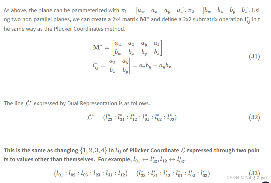
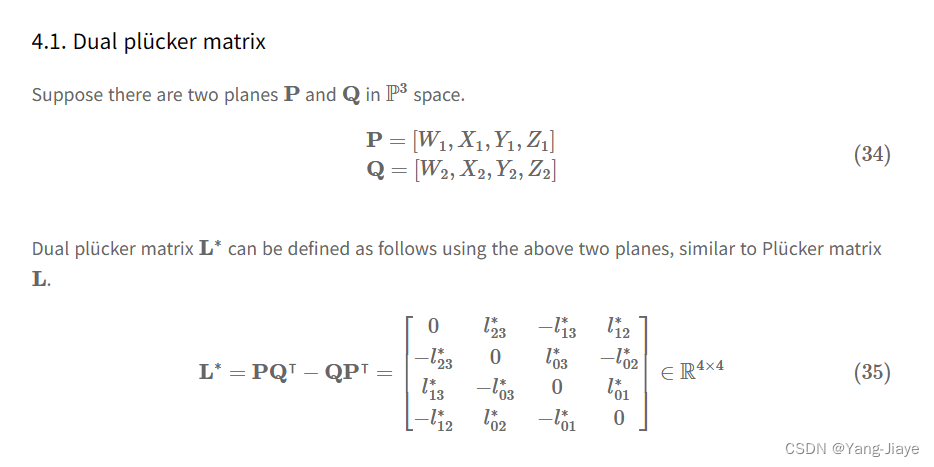
对偶Plucker坐标与矩阵

懒得码字了，直接贴图片吧，源自博客

投影矩阵的另一种构造

这是MVG书中给出的结论，里面用到了一个恒等式，我翻到73页的3.14，却发现作者没给证明QAQ。真是留图不留种，(…)

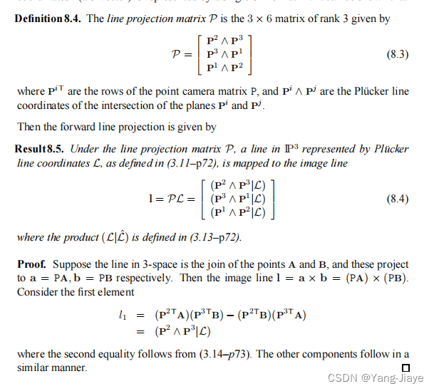
这里的外积是两个4维向量外积，所以得到的维数是$C_4^2=6$维，对应于$P=[R,R[-\mathbf{t}{]}_{\times }]$

参考文献

知乎1

知乎2

博客1

PL-VIO

[1] Camera Pose Estimation from Lines using Plücker Coordinates

[2] Development of a Navigation Solution for an Image Aided Automatic Landing System