gm/Id 设计方法

gm/Id方法的原理

关于gm/id设计方法的原理请看Stanford ee214b的课件。这两篇对基本原理已经讲的很详细，再次不过多阐述。本篇博客主要讲如何使用gm/Id方法。

简单概括gm/Id方法的本质就是：

• gm/Id对应Vov，通过其数值大小的选取来达到增益与带宽的折衷；
• gm/Id方法是一种loop-up table方法；
• gm/Id方法为短沟道器件电路设计提供了比公式手算更准确的初值；
• gm/Id方法为亚阈值设计提供了有力的工具。

原始数据准备

首先要在cadence或者hspice中通过大量参数扫描得到不同工作点下晶体管的小信号参数模型。此处以在cadence中得到tsmc180管子参数为例。

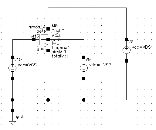
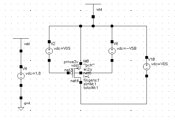
因为需要大量的仿真，并且导出的数据也很多，这里我们用ocean脚本来代替繁琐的操作。

注意：对于不会使用ocean语言的，可以通过这篇介绍 来快速的生成一个粗糙但不影响使用的ocean文件。

我的ocean代码如下：

simulator( 'spectre )
design(	 "/home/liuheng/simulation/NMOS2V_DC/spectre/schematic/netlist/netlist")
resultsDir( "/home/liuheng/simulation/NMOS2V_DC/spectre/schematic" )
modelFile(  
	'("/eda/library/TSMC/tsmc18rfOA/tsmc18/../models/spectre/cr018gpii_v1d0.scs" "stat_noise")
	。。。此处还有很多model，能自动生成，此处为了不影响博客的视觉效果删除了一些语句。
)
analysis('dc ?saveOppoint t  )
desVar(	  "L" 180n	)
desVar(	  "VDS" 0.9	)
desVar(	  "VGS" 0.9	)
desVar(	  "VSB" 0	)
envOption(
	'analysisOrder  list("dc") 
)
temp( 27 ) 


L_list = list(1.8e-07 2e-07 2.2e-07 2.4e-07 2.6e-07 2.8e-07 3e-07 3.2e-07 3.4e-07 3.6e-07 3.8e-07 4e-07 4.2e-07 4.4e-07 4.6e-07 4.8e-07 5e-07 5e-07 6e-07 7e-07 8e-07 9e-07 1e-06) 

VGS_list = list(0 0.1 0.2 0.3 0.4 0.5 0.6 0.7 0.8 0.9 1 1.1 1.2 1.3 1.4 1.5 1.6 1.7 1.8)

VDS_list = list(0 0.1 0.2 0.3 0.4 0.5 0.6 0.7 0.8 0.9 1 1.1 1.2 1.3 1.4 1.5 1.6 1.7 1.8)


paramAnalysis("L" ?values L_list
	paramAnalysis("VGS" ?values VGS_list
		paramAnalysis("VDS" ?values VDS_list
)))

paramRun()

para = list("gm" "gmbs" "id" "gds" "vth" "cgg" "css" "cjs" "cdd" "cjd" "cgd" "cgs" "cdb" "cds")

foreach(xx para 
	model = pv("M0" xx ?result "dcOpInfo-info")
	ocnPrint( ?output xx ?numberNotation 'scientific model )
)

数据处理

注意到我扫DC参数时也扫了VDS，导致得到的数据是3维的，不是很方便使用。

其实VDS变化带来的效应就是沟道长度调制效应，在模型方程中的体现就是 $\lambda$, 在小信号模型中的表现就是 $r_o$，其实我们大概推导以下公式就会发现：

g m I d = 2 μ C o x W / L I d ( 1 + λ V D S ) \frac{g_m}{I_d} = \sqrt{\frac{2\mu C_{ox} W/L}{I_d}(1+\lambda V_{DS})} I