


Background & Motivation
目标检测最开始采用滑窗的方法,深度学习兴起后二阶段检测模型占了主导地位,一阶段模型一直在追赶。文章认为一阶段检测模型精度不如二阶段检测模型的一个重要原因是前景/背景的比例失调,二阶段检测模型中使用 RPN、Selective Search、OHEM 等方法来应对这一问题,而一阶段的模型使用这些办法效果不是很好。前景/背景比例的失调会导致:
- 大多数的训练徘徊在 easy negative/well-classified example 上,使训练十分低效。
- 这些 easy negative/well-classified example 占用计算资源、主导了梯度下降,损害模型精度。
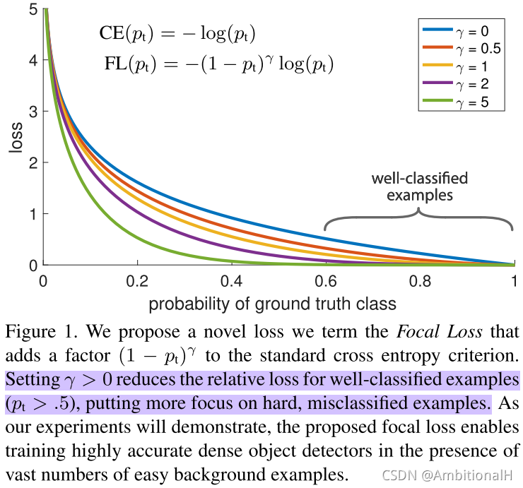
对于交叉熵损失函数(如下图中的蓝线),即使 well-classified example 也贡献了很多损失,当 well-classified example 数量很多时就主导了梯度下降,使模型不能更好的学习 hard example。
所以本文提出了 Focal Loss,使一阶段检测模型更加关注 hard example,也不需要像 OHEM 那样重新采样。
Focal Loss
对交叉熵损失函数进行改进,进一步区分 positive/negative example 来缓解比例失调的问题并作为本文的 baseline:
![]()
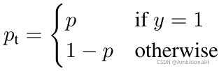
其中 αt 的定义与 pt 一样:
这个 αt 与 Faster Rcnn 中处理 positive/negative sample 比例失调的方法(第一阶段 RPN 过滤出2000个 proposal 以及将第二阶段中的 positive/negative proposal 比例为1:3)有着异曲同工之处,算是将这种方法用到了一阶段检测网络中。但是这种方法存在着不足:
While α balances the importance of positive/negative examples, it does not differentiate between easy/hard examples.
后续消融实验证明 αt 为0.25时与 γ 搭配起来效果最佳,按上述公式,αt 为0.25即正样本的权重为0.25,负样本权重的为0.75。正负样本权重比为1:3,与 RPN 中正负 proposal 数量的比例相同。
为了区分 esay/hard example,对损失函数 CE(pt) 再做改进也即 Focal Loss(positive/negative 的问题用 αt 应对,这里只关注 esay/hard):
![]()
γ 不同取值的损失曲线在上面的 Fig.1 中,log 前不带负号的部分为 modulating factor。随着 γ 的值增加,modulating factor 的影响也随之增加。
当 pt 的值很小(即置信度小,hard example),modulating factor 的值接近于1不影响损失的计算;而当 pt 很大接近1时(即有很大的置信度,对应那些 well-classified example),modulating factor 的值接近0。
We found γ = 2 to work best in our experiments.
Focal Loss 增大了 well-classified example 获得低 loss 的可能性,即尽可能地抑制掉 well-classified example。
将 Focal Loss 与 CE(pt) 结合得到 Focal Loss 的变体:
![]()
实验证明变体的效果要比其本身稍好一些,可以理解为 αt 用来调整 positive/negative sample,γ 用来调整 esay/hard example。
Finally, we note that the implementation of the loss layer combines the sigmoid operation for computing p with the loss computation, resulting in greater numerical stability.
22.01.13,一点新的理解。
Focal Loss 用在二阶段检测网络比如 Faster Rcnn 中没有起到平衡正负样本的作用,因为经过 RPN 后正负样本已经变为了1:3,在二阶段检测网络中 Focal Loss 的作用更多是难例挖掘。
真正彰显 Focal Loss 威力是在一阶段检测网络中,其正负样本极度不均衡。
RetinaNet

backbone
模型结构如上,将 FPN 和 ResNet 作为 backbone,都采用256个 channel,对 FPN 做了一定的改动:
We construct a pyramid with levels P3 through P7, where l indicates pyramid level (Pl has resolution
lower than the input).
RetinaNet uses feature pyramid levels P3 to P7, where P3 to P5 are computed from the output of the corresponding ResNet residual stage (C3 through C5) using top-down and lateral connections just as in FPN, P6 is obtained via a 3×3 stride-2 conv on C5, and P7 is computed by applying ReLU followed by a 3×3 stride-2 conv on P6. This differs slightly from FPN: (1) we don’t use the high-resolution pyramid level P2 for computational reasons, (2) P6 is computed by strided convolution instead of downsampling, and (3) we include P7 to improve large object detection. These minor modifications improve speed while maintaining accuracy.
Anchor
在中 FPN 的 P3 到 P7 上 anchor 的大小为32*32到512*512,以及
At each pyramid level we use anchors at three aspect ratios {1:2, 1:1, 2:1}. For denser scale coverage than in FPN, at each level we add anchors of sizes {
} of the original set of 3 aspect ratio anchors.
This improve AP in our setting. In total there are A = 9 anchors per level and across levels they cover the scale range 32 - 813 pixels with respect to the network’s input image.
在特征图上将 anchor 与 gt 计算IoU,大于0.5的为正样本,小于0.4的为负样本。
对 anchor 的尺度和长宽比进行了消融实验,其中 sc 为尺度的个数,ar 为长宽比的个数:
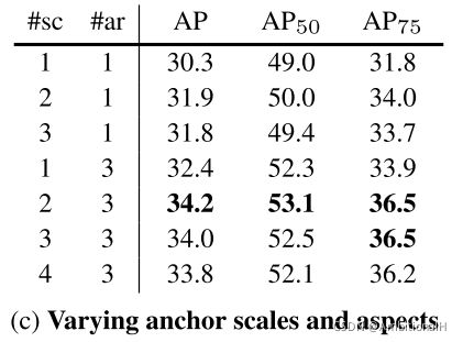
表中最后几行也证明增加 anchor 的数量并不能带来精度的提升。
Classification Head 和 Box Regression Head
两者的实现都是一个层数非常少的的 FCN(这两个 FCN 要比 Faster Rcnn 中 cls head、reg head 的层数更多一点),仅仅最后一层输出的通道数不同。各特征层的 cls head 和 reg head 都共享权重,并且这个 reg head 是 class-agnostic 的。
对 cls head 的最后一层卷积层的初始化也进行了精心的设计,将其偏置 b 初始化为:
![]()
这样可以避免在最开始训练的时候那些数量巨大的背景的 proposal 贡献大的损失,可以看作是应对前景/背景比例失调的一个 trick。下面是原文的解释,看的不是很懂:
Binary classification models are by default initialized to have equal probability of outputting either y = −1 or 1. Under such an initialization, inin the presence of class imbalance, the loss due to the frequent class can dominate total loss and cause instability in early training. To counter this, we introduce the concept of a ‘prior’ for the value of p estimated by the model for the rare class (foreground) at the start oftraining. We denote the prior by π and set it so that the model’s estimated p for examples of the rare class is low, e.g. 0.01. We found this to improve training stability for both the cross entropy and focal loss in the case of heavy class imbalance.
where π specifies that at the start of training every anchor should be labeled as foreground with confidence of ∼π.
We use π = 0.01 in all experiments, although results are robust to the exact value.
文中提到当用标准的交叉熵损失对 RetinaNet 训练时,很快就出现了梯度爆炸,模型开始发散。但是当加上这个初始化方法就可以将模型训练到收敛,在 COCO 数据集上获得了30.2%的准确率。
Loss Function
采用本文提出的 focal loss,在推理阶段为了加快速度 RPN 的每一层输出1000个 proposal,最后的 cls head 和 reg head 中聚合了所有尺度的预测并用阈值为0.5的 NMS 来过滤掉一定的预测。
而在训练时 focal loss 使 RetinaNet 可以使用每张 sampled image 的 RPN 中产生的所有 proposal(这些 proposal 被分配给 gt 的 anchor 的数量归一化),而不是用 OHEM 或者固定的超参数(Faster Rcnn)来输出256个proposal。
focal loss 中的超参数低的 α 搭配高的 γ 效果最好,实验证明 γ=2 和 α=0.25 时效果最好,总的损失函数为 focal loss + smooth L1(for box regression)。
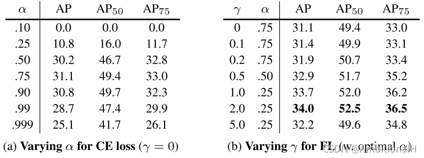
可以看出将上面的初始化方法加入到 CE(pt) 中,αt 设置为0.75时最高提升了0.9的 AP,前面提到将初始化方法加入到标准的交叉熵损失中 AP 为 30.2%。
Experiment
对 focal loss 进行了分析,在一批随机的图片中随机采样了10的5次方个正例和10的7次方个负例。算出这些采样的 focal loss 值,归一化后绘制其分布函数:
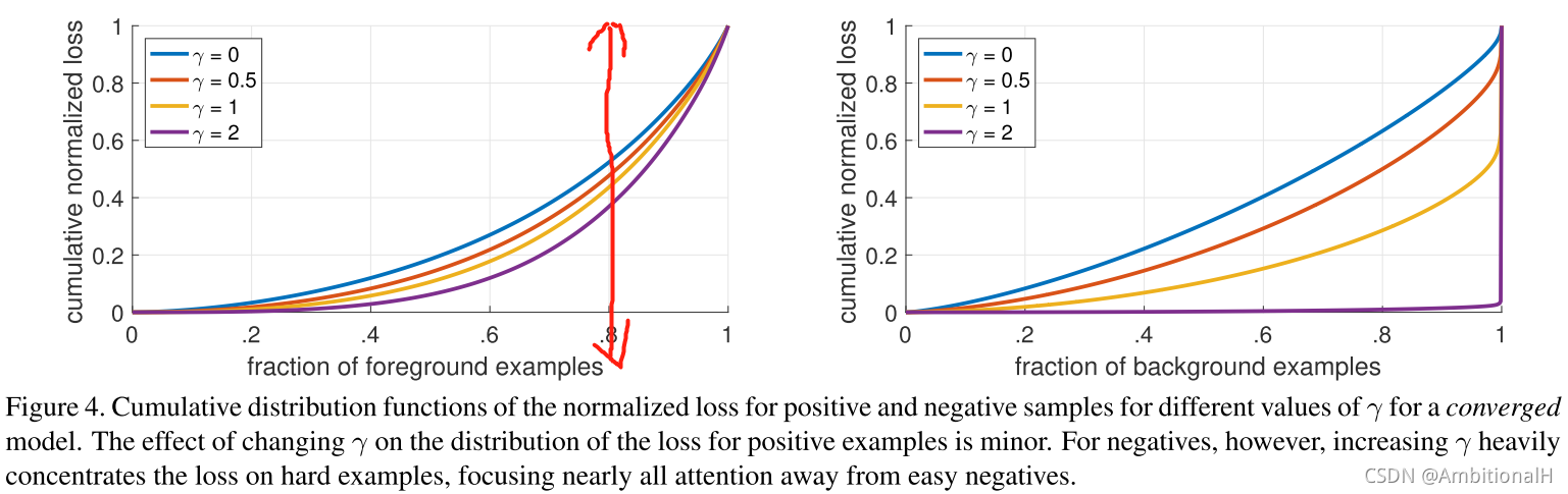
可以看出正例中随着 γ 的增加,20%的 proposal(红线右侧)贡献的损失越来越多(前面提到 γ 用来应对 esay/hard example,这里可以理解为更多的 hard example 贡献了更多的损失)。而对于负例随着 γ 的增加,几乎所有的损失都是由那些 hard example 来贡献(即 focal loss 可以用来使模型更关注 hard negative example)。
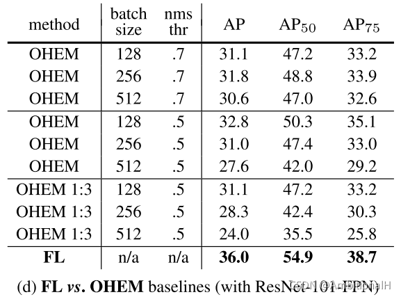
将 focal loss 与 OHEM 进行了比较,两者的不同在于后者完全放弃了那些 easy example。
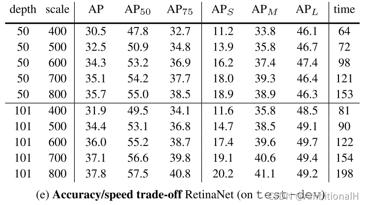
输入图像的尺度和推理时间都是模型两个很重要的性能:
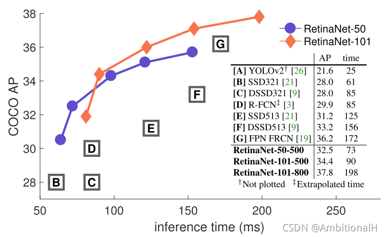
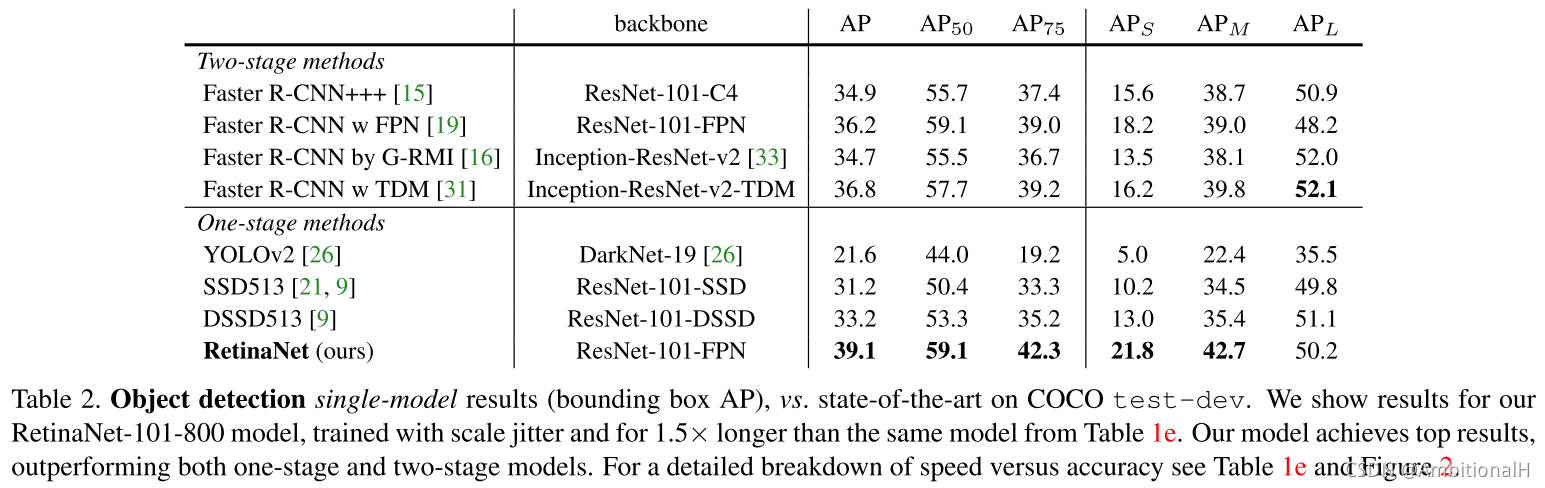
在 COCO 数据集上的精度:
Conclusion
focal loss 用在 cls head,用 focal loss 来缓解一阶段检测网络中的样本比例失衡的问题,文中还提出了对 cls head 初始化方法的一个 trick。
RetinaNet 中的 anchor 设置文章写的不是很清楚,用 FCN 来实现 cls head 和 reg head 的方法值得尝试。


 19万+
19万+

 被折叠的 条评论
为什么被折叠?
被折叠的 条评论
为什么被折叠?
 到【灌水乐园】发言


