自动驾驶常用数据集KITTI使用指南之一——图像雷达数据融合

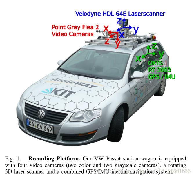
对于自动驾驶环境感知算法的初学者而言，一辆搭载各类传感器的自动驾驶汽车或者数据采集平台并没有那么重要，甚至，由于国外早期自动驾驶研究学者的严谨态度，一些公开的数据集比自己采集的数据集在同步性、针对性和多数据融合的匹配度等方面更加优良。（相比于初学者，对于自动驾驶汽车的研发工程师而言，在实际工程应用中，就应该注意数据保存的同步性、传感器的布局等细节，以造福感知算法研发者。）本文以著名的KITTI数据集中的Visual Odometry / SLAM Evaluation 2012数据子集使用为例，介绍视觉图像与三维雷达数据的融合使用。（在此感谢卡尔斯鲁厄理工学院（KIT）为自动驾驶研究者做出的贡献）本篇所用的数据集详细下载地址为：http://www.cvlibs.net/datasets/kitti/eval_odometry.php 。需要提前下载的数据集包括：image color、velodyne laser data、calibration files（此数据面向视觉里程计VO算法开发）。需要注意的问题是：KITTI数据集的坐标系为右手系，相对于车体局部坐标系而言，X轴为车辆行进前向，Y轴为横向，Z轴向上。

KITTI官网中有关于数据融合的matlab源码，但是对于以上数据集，并不能直接拿来用。原因在于给定的kit source code是以原始未矫正图像数据为处理对象，而文中的VO数据集是以矫正后的图像作为输入，因而内容处理上有所不同，需要进行相应的修改。本篇中matlab源代码参照了devkit中matlab源码设计，以devkit_odometry中readme.txt为依据，进行了代码的修改，下文为readme.txt中内容，可参阅。

###########################################################################
#   THE KITTI VISION BENCHMARK SUITE: VISUAL ODOMETRY / SLAM BENCHMARK    #
#              Andreas Geiger    Philip Lenz    Raquel Urtasun            #
#                    Karlsruhe Institute of Technology                    #
#                Toyota Technological Institute at Chicago                #
#                             www.cvlibs.net                              #
###########################################################################

This file describes the KITTI visual odometry / SLAM benchmark package.
Accurate ground truth (<10cm) is provided by a GPS/IMU system with RTK
float/integer corrections enabled. In order to enable a fair comparison of
all methods, only ground truth for the sequences 00-10 is made publicly
available. The remaining sequences (11-21) serve as evaluation sequences.

NOTE: WHEN SUBMITTING RESULTS, PLEASE STORE THEM IN THE SAME DATA FORMAT IN
WHICH THE GROUND TRUTH DATA IS PROVIDED (SEE 'POSES' BELOW), USING THE
FILE NAMES 11.txt TO 21.txt. CREATE A ZIP ARCHIVE OF THEM AND STORE YOUR
RESULTS IN ITS ROOT FOLDER.

File description:
=================

Folder 'sequences':

Each folder within the folder 'sequences' contains a single sequence, where
the left and right images are stored in the sub-folders image_0 and
image_1, respectively. The images are provided as greyscale PNG images and
can be loaded with MATLAB or libpng++. All images have been undistorted and
rectified. Sequences 0-10 can be used for training, while results must be
provided for the test sequences 11-21.

Additionally we provide the velodyne point clouds for point-cloud-based
methods. To save space, all scans have been stored as Nx4 float matrix into
a binary file using the following code:

  stream = fopen (dst_file.c_str(),"wb");
  fwrite(data,sizeof(float),4*num,stream);
  fclose(stream);

Here, data contains 4*num values, where the first 3 values correspond to
x,y and z, and the last value is the reflectance information. All scans
are stored row-aligned, meaning that the first 4 values correspond to the
first measurement. Since each scan might potentially have a different
number of points, this must be determined from the file size when reading
the file, where 1e6 is a good enough upper bound on the number of values:

  // allocate 4 MB buffer (only ~130*4*4 KB are needed)
  int32_t num = 1000000;
  float *data = (float*)malloc(num*sizeof(float));

  // pointers
  float *px = data+0;
  float *py = data+1;
  float *pz = data+2;
  float *pr = data+3;

  // load point cloud
  FILE *stream;
  stream = fopen (currFilenameBinary.c_str(),"rb");
  num = fread(data,sizeof(float),num,stream)/4;
  for (int32_t i=0; i<num; i++) {
    point_cloud.points.push_back(tPoint(*px,*py,*pz,*pr));
    px+=4; py+=4; pz+=4; pr+=4;
  }
  fclose(stream);

x,y and y are stored in metric (m) Velodyne coordinates.

IMPORTANT NOTE: Note that the velodyne scanner takes depth measurements
continuously while rotating around its vertical axis (in contrast to the cameras,
which are triggered at a certain point in time). This effect has been
eliminated from this postprocessed data by compensating for the egomotion!!
Note that this is in contrast to the raw data.

The relationship between the camera triggers and the velodyne is the following:
We trigger the cameras when the velodyne is looking exactly forward (into the
direction of the cameras). After compensation, the point cloud data should
correspond to the camera data for all static elements of the scene. Dynamic
ones are still slightly distorted, of course. If you want the raw velodyne
scans, please have a look at the section 'mapping to raw data' below.

The base directory of each folder additionally contains:

calib.txt: Calibration data for the cameras: P0/P1 are the 3x4 projection
matrices after rectification. Here P0 denotes the left and P1 denotes the
right camera. Tr transforms a point from velodyne coordinates into the
left rectified camera coordinate system. In order to map a point X from the
velodyne scanner to a point x in the i'th image plane, you thus have to
transform it like:

  x = Pi * Tr * X

times.txt: Timestamps for each of the synchronized image pairs in seconds,
in case your method reasons about the dynamics of the vehicle.

Folder 'poses':

The folder 'poses' contains the ground truth poses (trajectory) for the
first 11 sequences. This information can be used for training/tuning your
method. Each file xx.txt contains a N x 12 table, where N is the number of
frames of this sequence. Row i represents the i'th pose of the left camera
coordinate system (i.e., z pointing forwards) via a 3x4 transformation
matrix. The matrices are stored in row aligned order (the first entries
correspond to the first row), and take a point in the i'th coordinate
system and project it into the first (=0th) coordinate system. Hence, the
translational part (3x1 vector of column 4) corresponds to the pose of the
left camera coordinate system in the i'th frame with respect to the first
(=0th) frame. Your submission results must be provided using the same data
format.

Mapping to Raw Data
===================

Note that this section is additional to the benchmark, and not required for
solving the object detection task.

In order to allow the usage of the laser point clouds, gps data, the right
camera image and the grayscale images for the TRAINING data as well, we
provide the mapping of the training set to the raw data of the KITTI dataset.
The following table lists the name, start and end frame of each sequence that
has been used to extract the visual odometry / SLAM training set:

Nr.     Sequence name     Start   End
---------------------------------------
00: 2011_10_03_drive_0027 000000 004540
01: 2011_10_03_drive_0042 000000 001100
02: 2011_10_03_drive_0034 000000 004660
03: 2011_09_26_drive_0067 000000 000800
04: 2011_09_30_drive_0016 000000 000270
05: 2011_09_30_drive_0018 000000 002760
06: 2011_09_30_drive_0020 000000 001100
07: 2011_09_30_drive_0027 000000 001100
08: 2011_09_30_drive_0028 001100 005170
09: 2011_09_30_drive_0033 000000 001590
10: 2011_09_30_drive_0034 000000 001200

The raw sequences can be downloaded from
http://www.cvlibs.net/datasets/kitti/raw_data.php
in the respective category (mostly: Residential).

Evaluation Code:
================

For transparency we have included the KITTI evaluation code in the
subfolder 'cpp' of this development kit. It can be compiled via:

g++ -O3 -DNDEBUG -o evaluate_odometry evaluate_odometry.cpp matrix.cpp

根据devkit_odometry中readme.txt中所述：雷达点云是以二进制形式存储，后缀为.bin，每行数据表示一个雷达点：x y z intensity，其中(x,y,z)单位为米，intensity为回波强度，范围在0~1.0之间。回波强度大小与雷达距离物体的远近和物体本身的反射率有关，一般情况下应用不到，此处可以忽略此列内容。图像数据是以.png格式存储，可直接查看。图像已经进行了畸变矫正，在此以双目视觉的左图像为例，进行雷达点云与图像数据的融合处理。

三维点云到图像平面的投影变换过程，可从下图得到直观的印象：将物理世界中三维信息投影到一定视角下的二维信息（浅粉色平面），投影变换是以牺牲深度信息为代价的（复杂的公式推导详见投影变换的相关内容讲解，此处只提供快速工程化应用方法）。

KITTI中雷达点云与图像的配准关系存放在calib.txt中，其转换关系为：

其中，为3*4的投影矩阵，为3*4的变换矩阵，表示雷达点云到图像坐标系的平移变换。为保证矩阵运算的数据对齐，将矩阵补充为欧式变换矩阵，。当然，公式简化了投影变换的处理，实际投影变换过程中的matlab源码如下：

velo_img = project(velo(:,1:3), calib.P0*calib.TrRT);


function p_out = project(p_in,T)

% dimension of data and projection matrix

dim_norm = size(T,1);

dim_proj = size(T,2);

% do transformation in homogenuous coordinates

p2_in = p_in;

if size(p2_in,2)<dim_proj

  p2_in(:,dim_proj) = 1;

end

p2_out = (T*p2_in')';

% normalize homogeneous coordinates:

p_out = p2_out(:,1:dim_norm-1)./(p2_out(:,dim_norm)*ones(1,dim_norm-1));

velo_img存放着三维点云投影到图像平面的结果，如图所示：

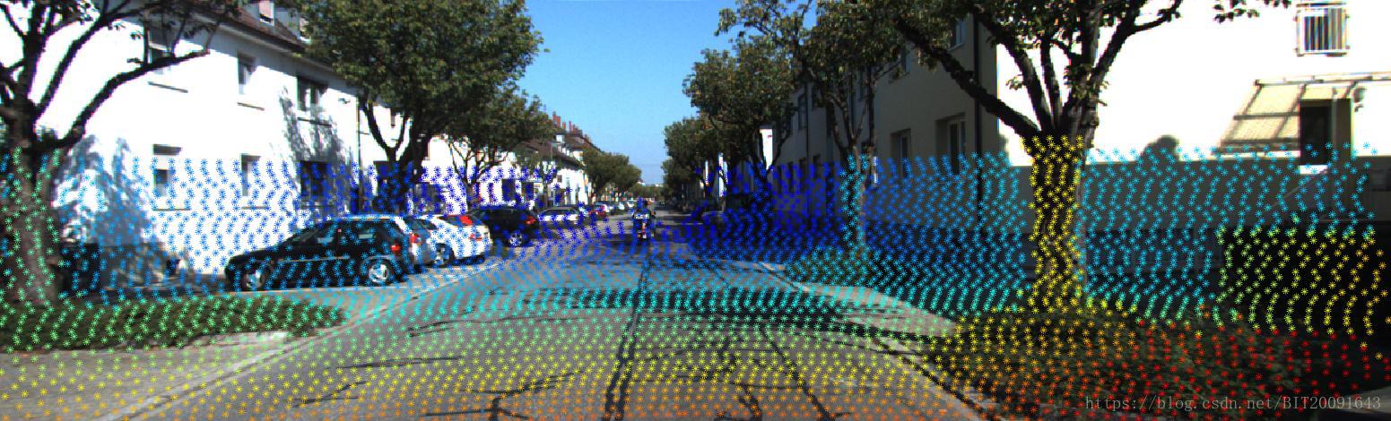
图中，点阵的颜色表示景深，暖色调表示近距，冷色调表示远距。

数据融合的好处在于兼顾了三维雷达点云的空间分布信息和图像的色彩信息，提供了图像分割、目标识别等问题求解的感兴趣区域，简化了问题研究难度，同时提高了待处理问题的数据维度，有利于机器学习、深度学习的细化分类。

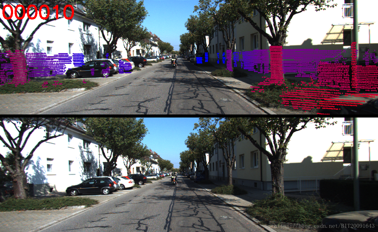
对于雷达点云有一定算法研究的同学，也可以通过去除地面点云和空间聚类分析等方法，实现物体分类。下图所示为去除地面点云后的障碍物分布。其中，树干、电线杆、汽车等物体被有效的分割成独立的感兴趣区域，降低了图像搜索的空间复杂度，对于目前比较流行的基于语义理解的环境建模等提供了物体分割依据。

数据融合处理，可以整合不同传感器优势所在，是目前比较流行的环境感知处理方法，包括目标识别、视觉里程计等，都可以通过二者的结合，发挥更好的效果。文中完整代码的下载地址为：https://download.csdn.net/download/bit20091643/10559805 。没有下载币的也可以私信我，希望本篇可以帮助到正在初学路上的自动驾驶爱好者。