


目录
(一):整体介绍
一、优缺点分析
通过实测和阅读代码,它有如下优缺点:
- 优点
1)简洁的流程和代码结构。
激光slam虽然相对简单,但是目前开源的算法里,能够同时融合gps、imu、lidar三种传感器的还比较少。cartographer算是一种,但是相对于它来讲,hdl_graph_slam在资源消耗、代码复杂度、建图流程等方面还是有很大优势。
2)增加地面检测。
当所处的环境中地面为平面时,它就可以作为一个很有效的信息去约束高程的误差,而做过激光slam的都知道,在没有gps的情况下,高程误差是主要的误差项。当然在地面为非平面的时候是不能够使用的,但这不能作为它的缺点,而应该在使用时根据环境决定是否开启这项功能。
3)具有闭环检测功能
闭环检测是slam中的重要功能,不只在没有gps参考的情况下能减小累计误差,即便在有gps约束的情况下也能起到有效的作用,而这一点却是很容易被忽略的地方。很多人认为有了gps就可以不使用闭环修正了,而大量的实验结果表明,这是非常错误的想法。
- 缺点
1)点云匹配精度不高。
这包括前端帧间匹配和闭环检测时的匹配,具体原因我们会在后面介绍到相应的代码时再讲。
二、功能分解
对整套系统的功能进行分解是为了能够更清晰的分析代码。这套系统的内部共包含四个主要功能项,所有的代码也是围绕着这四项功能展开的,它们分别是:
-
地面平面检测
根据点云检测平面,并拟合平面得到平面的数学描述参数,供构建概率图使用。 -
点云滤波
处理原始点云,得到稀疏点云 -
前端里程计
帧间匹配,得到每一帧位姿 -
后端概率图构建
这一项功能承担了整个系统中的大部分内容,它的主要功能又包括:
1)提取关键帧。
前端里程计得到的是每一帧位姿,而构建概率图只需要每隔一段距离取一帧就行,即关键帧。
2)读取gps、imu信息并加入概率图。
即使用gps、imu信息构建对应的边。
3)读取地面检测参数并加入概率图。
同样是构建边,只不过信息变了。
4)检测闭环,若成功,则加入概率图。
同样是构建边。
三、代码结构
完成上面的功能分析,我们就好分析代码了,因为代码是围绕功能展开的,而且代码结构和功能对应的很好,很清晰。
我们看下工程目录中主要文件夹及其内容:
- apps:节点文件
节点文件就是生成可执行文件的代码文件,相当于整个程序的入口。对应上面四项功能,它也就有了四个.cpp文件,分别是:
floor_detection_nodelet.cpp:地面平面检测
prefiltering_nodelet.cpp:点云滤波
scan_matching_odometry_nodelet.cpp:前端里程计
hdl_graph_slam_nodelet.cpp:后端概率图构建
2. include:头文件
头文件又包含两个文件夹:
1)g2o
定义了各信息源对应的g2o中的边。因为很多信息在g2o中没有对应的边,需要自己定义。
具体定义了哪些边,我们会在后面详细介绍。
2)hdl_graph_slam
全部四项功能都在这个文件夹中,它包含以下文件:
graph_slam.hpp:管理graph,即负责对概率图添加顶点和边。
information_matrix_calculator:计算信息矩阵,信息矩阵即是概率图中边的权重。
keyframe_updater:检测关键帧
keyframe:关键帧对应的结构
loop_detector:检测闭环
map_cloud_generator:生成地图点云,即是拼接地图
nmea_sentence_parser:处理gps信息,从nmea报文得到经纬高数据
registrations:设置点云匹配方法(程序中给了多种方法供选择,此处是指定选择哪一种)
ros_time_hash:管理rostime的小工具函数
ros_utils:各类位姿矩阵表示形式之间转换的工具函数
3. src:源文件
它包含的所有cpp文件在include中都有对应的头文件,而他们的功能在include中已经介绍过了,所以我们不在此列出了,详细内容后面的文章会介绍。
(二):g2o顶点和边的管理
一、整体分析
通过上一篇分析我们知道,在整个系统中,需要用来构建g2o的顶点或边的信息包括:
帧间匹配的位姿
闭环检测的位姿
gps的经纬高
imu的姿态
检测并拟合出的地面平面参数
本篇的主要内容就是分析这些信息对应的顶点和边是怎样定义的,并且在信息到来时,是怎样被添加到概率图中的。
这里面除了帧间匹配得到的位姿对应的顶点和边不需要自己定义以外,其他信息对应的边都需要自己定义,所谓自己定义就是从g2o中继承边对应的基类,产生一个子类,在该子类中写明这个边对应的信息矩阵和观测误差计算公式即可。
对于自定义的边,在该系统中,他们的使用遵循下面的流程:
1)在include/g2o中定义边。这个文件夹有很多个cpp文件,每个cpp文件对应一种类型的边。
2)在src/hdl_graph_slam/graph_slam.cpp处理边。所谓处理,是指边的插入,边往概率图中插入时需要完成多个步骤,在这个cpp文件里,每条边对应一个函数,把这多个步骤都封装在这个函数中,使用只需要调用一次函数即可,这样可使代码更清晰明了。
3)在apps/hdl_graph_slam_nodelet.cpp中调用边。所有的边都是在这个cpp文件中被加入概率图中的,当一个信息到来,需要添加边时,就调用2)中封装好的对应的函数就好了。
二、详解顶点和边
在这部分,我们根据文章开头列出的信息,按照顺序分析他们在g2o中对应的顶点和边。
每个元素(即顶点或边)对应一个函数,所有元素的管理函数都在src/hdl_graph_slam/graph_slam.cpp中,而管理函数的调用都在apps/hdl_graph_slam_nodelet.cpp中,所以后面我提函数和函数调用的代码的时候就不注明它们出自哪个文件了
- 帧间匹配的位姿
帧间匹配的位姿包括每一帧点云采集完成时雷达的位姿,以及相邻两帧点云之间的相对位姿,需要注意的是,我们构建概率图当然是稀疏的,不可能每一帧点云都参与,所以此处的帧均指关键帧,关键帧的选取策略后面会仔细讲。
在此处雷达自身的位姿即是顶点,而相邻两关键帧之间的相对位姿即是边。我们要分别介绍
1)顶点
添加顶点的函数代码如下
g2o::VertexSE3* GraphSLAM::add_se3_node(const Eigen::Isometry3d& pose) {
  g2o::VertexSE3* vertex(new g2o::VertexSE3());//定义并初始化一个顶点
  vertex->setId(static_cast<int>(graph->vertices().size()));//顶点对应的编号
  vertex->setEstimate(pose);//顶点对应的位姿
  graph->addVertex(vertex);//添加顶点到图中

  return vertex;
}
代码里VertexSE3是g2o中默认存在的顶点类型,它包括位置信息和姿态信息。
graph就是整个概率图,后面出现这个变量都是指这个意思,不再重复。
添加顶点时执行如下流程
Eigen::Isometry3d odom = odom2map * keyframe->odom;
keyframe->node = graph_slam->add_se3_node(odom);
keyframe_hash[keyframe->stamp] = keyframe;
2)边
添加边的函数代码如下
g2o::EdgeSE3* GraphSLAM::add_se3_edge(g2o::VertexSE3* v1, g2o::VertexSE3* v2, const Eigen::Isometry3d& relative_pose, const Eigen::MatrixXd& information_matrix) {
  g2o::EdgeSE3* edge(new g2o::EdgeSE3());//定义并初始化一条边
  edge->setMeasurement(relative_pose);//设置边对应的观测
  edge->setInformation(information_matrix);//设置信息矩阵
  edge->vertices()[0] = v1;//设置边的一端连接的顶点
  edge->vertices()[1] = v2;//设置边的另一端连接的顶点
  graph->addEdge(edge);//添加边到图中

  return edge;
}
调用流程如下
Eigen::Isometry3d relative_pose = keyframe->odom.inverse() * prev_keyframe->odom;
Eigen::MatrixXd information = inf_calclator->calc_information_matrix(prev_keyframe->cloud, keyframe->cloud, relative_pose);
auto edge = graph_slam->add_se3_edge(keyframe->node, prev_keyframe->node, relative_pose, information);
graph_slam->add_robust_kernel(edge, private_nh.paramstd::string(“odometry_edge_robust_kernel”, “NONE”), private_nh.param(“odometry_edge_robust_kernel_size”, 1.0));
2. 闭环检测的位姿
变换检测就不需要添加顶点了,只需要添加边。因为闭环是在关键帧中间进行检测的,在进行检测时,每个关键帧已经有对应的顶点加入图中了。
闭环的边和帧间匹配的边类型一样,不再重复了。
- gps的经纬高
gps能在建图时使用的是位置信息,也就是经度、纬度、高度,相当于给顶点(包含位置和姿态)中的位置信息一个直接的先验观测,也即先验边(prior)名称的由来。当然在添加到图中之前,会先把经度、纬度、高度转换到以地图原点为起始点的坐标系中,变成以米为单位的距离表示。
有些时候,如果认为高度不准,还可以只使用经度、纬度,而不使用高度,所以就有了下面这两种类型的边。
1)经度、纬度、高度同时观测
这是一个自定义的边,自定义对应的代码在include/g2o/edge_se3_priorxyz.hpp中,大家自己去看吧,应该都能看懂,不需要解释。
元素管理对应的函数代码如下
g2o::EdgeSE3PriorXYZ* GraphSLAM::add_se3_prior_xyz_edge(g2o::VertexSE3* v_se3, const Eigen::Vector3d& xyz, const Eigen::MatrixXd& information_matrix) {
g2o::EdgeSE3PriorXYZ* edge(new g2o::EdgeSE3PriorXYZ());//定义并初始化
edge->setMeasurement(xyz);//设置观测
edge->setInformation(information_matrix);//添加信息矩阵
edge->vertices()[0] = v_se3;//设置对应的顶点
graph->addEdge(edge);//添加边到图中
return edge;
}
调用流程如下
Eigen::Matrix2d information_matrix = Eigen::Matrix2d::Identity() / gps_edge_stddev_xy;
edge = graph_slam->add_se3_prior_xy_edge(keyframe->node, xyz.head<2>(), information_matrix);
2)经度、纬度观测
自定义边对应的代码在include/g2o/edge_se3_priorxy.hpp中
元素管理中,无非是向量少了一个维度嘛,和1)中的比变化不大
g2o::EdgeSE3PriorXY* GraphSLAM::add_se3_prior_xy_edge(g2o::VertexSE3* v_se3, const Eigen::Vector2d& xy, const Eigen::MatrixXd& information_matrix) {
g2o::EdgeSE3PriorXY* edge(new g2o::EdgeSE3PriorXY());//定义并初始化
edge->setMeasurement(xy);//设置观测(这里少了一个维度)
edge->setInformation(information_matrix);//添加信息矩阵
edge->vertices()[0] = v_se3;//设置对应的顶点
graph->addEdge(edge);//添加边到图中
return edge;
}
调用流程如下
Eigen::Matrix3d information_matrix = Eigen::Matrix3d::Identity();
information_matrix.block<2, 2>(0, 0) /= gps_edge_stddev_xy;
information_matrix(2, 2) /= gps_edge_stddev_z;
edge = graph_slam->add_se3_prior_xyz_edge(keyframe->node, xyz, information_matrix);
- imu的角度和加速度
在这个系统中,使用了imu的角度和加速度信息,角度自然就是给位姿做角度观测(四元数形式),而加速度,则是以重力作为基准方向,计算imu检测的加速度矢量和重力的不重合度,并作为误差项进行优化。
因此imu信息也对应两类边
1)角度信息
自定义边的代码在include/g2o/edge_se3_priorquat.hpp中
元素管理的代码如下
g2o::EdgeSE3PriorQuat* GraphSLAM::add_se3_prior_quat_edge(g2o::VertexSE3* v_se3, const Eigen::Quaterniond& quat, const Eigen::MatrixXd& information_matrix) {
g2o::EdgeSE3PriorQuat* edge(new g2o::EdgeSE3PriorQuat());//定义并初始化
edge->setMeasurement(quat);//添加观测
edge->setInformation(information_matrix);//添加信息矩阵
edge->vertices()[0] = v_se3;//指定顶点
graph->addEdge(edge);//添加边到图中
return edge;
}
调用的代码如下
Eigen::MatrixXd info = Eigen::MatrixXd::Identity(3, 3) / imu_orientation_edge_stddev;
auto edge = graph_slam->add_se3_prior_quat_edge(keyframe->node, *keyframe->orientation, info);
graph_slam->add_robust_kernel(edge, private_nh.param<std::string>("imu_orientation_edge_robust_kernel", "NONE"), private_nh.param<double>("imu_orientation_edge_robust_kernel_size", 1.0));
2)加速度信息
自定义边的代码在include/g2o/edge_se3_priorvec.hpp中
元素管理的代码如下
g2o::EdgeSE3PriorVec* GraphSLAM::add_se3_prior_vec_edge(g2o::VertexSE3* v_se3, const Eigen::Vector3d& direction, const Eigen::Vector3d& measurement, const Eigen::MatrixXd& information_matrix) {
  Eigen::Matrix<double, 6, 1> m;
  m.head<3>() = direction;
  m.tail<3>() = measurement;

  g2o::EdgeSE3PriorVec* edge(new g2o::EdgeSE3PriorVec());
  edge->setMeasurement(m);
  edge->setInformation(information_matrix);
  edge->vertices()[0] = v_se3;
  graph->addEdge(edge);

  return edge;
}
上面direction就是参考方向,而measurement就是测量的方向。这个边的误差就是这两个向量的差。
调用代码如下
Eigen::MatrixXd info = Eigen::MatrixXd::Identity(3, 3) / imu_acceleration_edge_stddev;
g2o::OptimizableGraph::Edge* edge = graph_slam->add_se3_prior_vec_edge(keyframe->node, -Eigen::Vector3d::UnitZ(), *keyframe->acceleration, info);
graph_slam->add_robust_kernel(edge, private_nh.param<std::string>("imu_acceleration_edge_robust_kernel", "NONE"), private_nh.param<double>("imu_acceleration_edge_robust_kernel_size", 1.0));
上面参考方向设置为-Eigen::Vector3d::UnitZ(),即重力方向,测量方向设置为acceleration,即测量的加速度方向,所以这条边的误差就变成了加速度和重力之间的误差,和上面的分析一致。
- 平面检测的信息
我们知道平面的方程是ax + by + cz + d=0,所以一个平面(plane)可以由四个参数描述。平面在这里既用来构造顶点,又参与构造边,所以元素分下面两类
1)顶点
平面对应的顶点在g2o中本来就有(g2o::VertexPlane),所以不需要自己定义。
元素管理对应的代码如下
g2o::VertexPlane* GraphSLAM::add_plane_node(const Eigen::Vector4d& plane_coeffs) {
  g2o::VertexPlane* vertex(new g2o::VertexPlane());
  vertex->setId(static_cast<int>(graph->vertices().size()));
  vertex->setEstimate(plane_coeffs);
  graph->addVertex(vertex);

  return vertex;
}
调用的代码如下
floor_plane_node = graph_slam->add_plane_node(Eigen::Vector4d(0.0, 0.0, 1.0, 0.0));
floor_plane_node->setFixed(true);
我们看到,添加VertexPlane类型的顶点在程序中只出现了一次,而且平面参数直接被设置成了 Eigen::Vector4d(0.0, 0.0, 1.0, 0.0),这其实就是在初始化位姿的时候添加的,认为载体处在一个平面上,才能有这样的假设成立。
2)边
平面对应的边是自定义的,对应的代码在include/g2o/edge_se3_plane.hpp文件中
元素管理的代码如下
g2o::EdgeSE3Plane* GraphSLAM::add_se3_plane_edge(g2o::VertexSE3* v_se3, g2o::VertexPlane* v_plane, const Eigen::Vector4d& plane_coeffs, const Eigen::MatrixXd& information_matrix) {
  g2o::EdgeSE3Plane* edge(new g2o::EdgeSE3Plane());
  edge->setMeasurement(plane_coeffs);
  edge->setInformation(information_matrix);
  edge->vertices()[0] = v_se3;
  edge->vertices()[1] = v_plane;
  graph->addEdge(edge);

  return edge;
}
调用的代码如下
Eigen::Vector4d coeffs(floor_coeffs->coeffs[0], floor_coeffs->coeffs[1], floor_coeffs->coeffs[2], floor_coeffs->coeffs[3]);
Eigen::Matrix3d information = Eigen::Matrix3d::Identity() * (1.0 / floor_edge_stddev);
auto edge = graph_slam->add_se3_plane_edge(keyframe->node, floor_plane_node, coeffs, information);
graph_slam->add_robust_kernel(edge, private_nh.param<std::string>("floor_edge_robust_kernel", "NONE"), private_nh.param<double>("floor_edge_robust_kernel_size", 1.0));
我们看到,这种操作把所有的关键帧对应的顶点都和初始化的平面(即Eigen::Vector4d(0.0, 0.0, 1.0, 0.0))建立了联系,相当于把整个slam系统约束在平面上,认为它是在沿平面移动。
所以这种边要不要加需要根据环境决定,如果环境符合假设,那么高程几乎没有误差(我试过),如果不符合,那么相当于引入了错误的约束,会增大误差,甚至导致地图错乱。
至此所有的顶点和边就介绍完了。
其实在g2o文件夹中还有其他自定义的边,在src/hdl_graph_slam/graph_slam.cpp中还有其他元素管理函数,他们是有用的,但是本系统并没有调用,所以暂时不做过多解释了。
三、信息矩阵
细心的读者应该已经从上面的代码中发现,我们每次添加一条边的时候都要给出相应的信息矩阵,它反应的是这条边在优化中的权重,实际中,如果觉得优化结果不太好,我们可以根据实际情况去调整这些权重以取得更好的效果。
既然每种边都有权重,那我们就按照边的类型来梳理一下对应的信息矩阵。
- 帧间匹配的位姿
它添加边的代码如下
Eigen::Isometry3d relative_pose = keyframe->odom.inverse() * prev_keyframe->odom;
Eigen::MatrixXd information = inf_calclator->calc_information_matrix(prev_keyframe->cloud, keyframe->cloud, relative_pose);
auto edge = graph_slam->add_se3_edge(keyframe->node, prev_keyframe->node, relative_pose, information);
我们从上面的代码可以看出,它的信息矩阵是通过calc_information_matrix这个函数计算的,这个函数在文件src/hdl_graph_slam/information_matrix_calculator.cpp中,我们看下它的具体代码
Eigen::MatrixXd InformationMatrixCalculator::calc_information_matrix(const pcl::PointCloud<PointT>::ConstPtr& cloud1, const pcl::PointCloud<PointT>::ConstPtr& cloud2, const Eigen::Isometry3d& relpose) const {
  if(use_const_inf_matrix) {
    Eigen::MatrixXd inf = Eigen::MatrixXd::Identity(6, 6);
    inf.topLeftCorner(3, 3).array() /= const_stddev_x;
    inf.bottomRightCorner(3, 3).array() /= const_stddev_q;
    return inf;
  }

  double fitness_score = calc_fitness_score(cloud1, cloud2, relpose);//计算匹配程度

  double min_var_x = std::pow(min_stddev_x, 2);
  double max_var_x = std::pow(max_stddev_x, 2);
  double min_var_q = std::pow(min_stddev_q, 2);
  double max_var_q = std::pow(max_stddev_q, 2);

  //根据匹配程度计算权重,位置权重和姿态权重分别计算
  float w_x = weight(var_gain_a, fitness_score_thresh, min_var_x, max_var_x, fitness_score);
  float w_q = weight(var_gain_a, fitness_score_thresh, min_var_q, max_var_q, fitness_score);

  Eigen::MatrixXd inf = Eigen::MatrixXd::Identity(6, 6);
  inf.topLeftCorner(3, 3).array() /= w_x;
  inf.bottomRightCorner(3, 3).array() /= w_q;
  return inf;
}
可以看出,整个计算过程分为两步,第一步是计算两帧点云的匹配程度,也就是位姿的准确程度(因为位姿越不准,点云的匹配重合度就越差呀),第二步就是根据第一步的结果,计算信息矩阵里的值。
我们对这两步分别分析
1)计算匹配程度
直接上代码
double InformationMatrixCalculator::calc_fitness_score(const pcl::PointCloud<PointT>::ConstPtr& cloud1, const pcl::PointCloud<PointT>::ConstPtr& cloud2, const Eigen::Isometry3d& relpose, double max_range) {
  pcl::search::KdTree<PointT>::Ptr tree_(new pcl::search::KdTree<PointT>());
  tree_->setInputCloud(cloud1);

  double fitness_score = 0.0;

  // Transform the input dataset using the final transformation
  pcl::PointCloud<PointT> input_transformed;
  pcl::transformPointCloud (*cloud2, input_transformed, relpose.cast<float>());

  std::vector<int> nn_indices (1);
  std::vector<float> nn_dists (1);

  // For each point in the source dataset
  int nr = 0;
  for (size_t i = 0; i < input_transformed.points.size (); ++i)
  {
    // Find its nearest neighbor in the target
    tree_->nearestKSearch (input_transformed.points[i], 1, nn_indices, nn_dists);

    // Deal with occlusions (incomplete targets)
    if (nn_dists[0] <= max_range)
    {
      // Add to the fitness score
      fitness_score += nn_dists[0];
      nr++;
    }
  }

  if (nr > 0)
    return (fitness_score / nr);
  else
    return (std::numeric_limits<double>::max ());
}
可以看出,它的思路就是对于当前点云中的每一个点,在另一帧点云中找最近的点,如果这两点之间的距离在合理范围内,则把他俩之间的距离差作为不匹配度的误差加如最终的fitness_score中。
2)计算权重
这里要问,既然有了fitness了,为什么直接把它当权重不行吗,为什么还要进行一次计算呢。因为fitness的变化范围比较大,而且fitness和不匹配度只是正相关关系,而其曲线分布并不合理,所以要重新改变曲线形状。
就是下面这个函数
double weight(double a, double max_x, double min_y, double max_y, double x) const {
double y = (1.0 - std::exp(-a * x)) / (1.0 - std::exp(-a * max_x));
return min_y + (max_y - min_y) * y;
}
而这一步所需要参数是从launch文件里传入的,也就是使用者可以通过配置参数来更改。
-
闭环检测的位姿
都属于点云匹配得到的边,所以计算方式和帧间匹配的边是一样的。 -
gps的经纬高
1)经度、纬度、高度同时观测
Eigen::Matrix3d information_matrix = Eigen::Matrix3d::Identity();
information_matrix.block<2, 2>(0, 0) /= gps_edge_stddev_xy;
information_matrix(2, 2) /= gps_edge_stddev_z;
edge = graph_slam->add_se3_prior_xyz_edge(keyframe->node, xyz, information_matrix);
可以看出,信息矩阵是通过gps_edge_stddev_xy和gps_edge_stddev_z两个参数直接计算的,前者代表经度、纬度的权重,后者代表高度的权重。使用者同样可以通过配置文件直接更改这两个参数。
2)经度、纬度观测
Eigen::Matrix2d information_matrix = Eigen::Matrix2d::Identity() / gps_edge_stddev_xy;
edge = graph_slam->add_se3_prior_xy_edge(keyframe->node, xyz.head<2>(), information_matrix);
少了高度而已,不用解释。
- imu的角度和加速度
1)imu角度信息
Eigen::MatrixXd info = Eigen::MatrixXd::Identity(3, 3) / imu_orientation_edge_stddev;
auto edge = graph_slam->add_se3_prior_quat_edge(keyframe->node, *keyframe->orientation, info);
同样从配置文件的参数直接计算,不解释
2)imu加速度信息
Eigen::MatrixXd info = Eigen::MatrixXd::Identity(3, 3) / imu_acceleration_edge_stddev;
g2o::OptimizableGraph::Edge* edge = graph_slam->add_se3_prior_vec_edge(keyframe->node, -Eigen::Vector3d::UnitZ(), *keyframe->acceleration, info);
同上
四、鲁棒核
在g2o中添加边时,如果添加鲁棒核,则系统会对一些异常数据更鲁棒,这套代码中,所有的边后面都跟了添加鲁棒核的操作。
其实就是调用了这个函数
void GraphSLAM::add_robust_kernel(g2o::HyperGraph::Edge* edge, const std::string& kernel_type, double kernel_size) {
if(kernel_type == “NONE”) {
return;
}
g2o::RobustKernel* kernel = robust_kernel_factory->construct(kernel_type);
if(kernel == nullptr) {
std::cerr << "warning : invalid robust kernel type: " << kernel_type << std::endl;
return;
}
kernel->setDelta(kernel_size);
g2o::OptimizableGraph::Edge* edge_ = dynamic_castg2o::OptimizableGraph::Edge*(edge);
edge_->setRobustKernel(kernel);
}
鲁棒核的类型可以在配置文件里设置,每种边都对应了一个设置变量,即他们各自的鲁棒核可以分别设置。
(三):点云滤波
点云滤波的内容主要在apps/prefiltering_nodelet.cpp中,主要包括两步滤波,一是降采样,而是滤除离群点,我们分别介绍。
1. 降采样滤波
降采样滤波的代码如下
// select a downsample method (VOXELGRID, APPROX_VOXELGRID, NONE)
std::string downsample_method = pnh.paramstd::string(“downsample_method”, “VOXELGRID”);
double downsample_resolution = pnh.param(“downsample_resolution”, 0.1);
if(downsample_method == “VOXELGRID”) {
std::cout << "downsample: VOXELGRID " << downsample_resolution << std::endl;
boost::shared_ptr<pcl::VoxelGrid> voxelgrid(new pcl::VoxelGrid());
voxelgrid->setLeafSize(downsample_resolution, downsample_resolution, downsample_resolution);
downsample_filter = voxelgrid;
} else if(downsample_method == “APPROX_VOXELGRID”) {
std::cout << “downsample: APPROX_VOXELGRID " << downsample_resolution << std::endl;
boost::shared_ptr<pcl::ApproximateVoxelGrid> approx_voxelgrid(new pcl::ApproximateVoxelGrid());
approx_voxelgrid->setLeafSize(downsample_resolution, downsample_resolution, downsample_resolution);
downsample_filter = approx_voxelgrid;
} else {
if(downsample_method != “NONE”) {
std::cerr << “warning: unknown downsampling type (” << downsample_method << “)” << std::endl;
std::cerr << " : use passthrough filter” <<std::endl;
}
std::cout << “downsample: NONE” << std::endl;
boost::shared_ptr<pcl::PassThrough> passthrough(new pcl::PassThrough());
downsample_filter = passthrough;
}
这段代码的内容也比较清晰,它先从配置文件中读取参数downsample_method,根据参数决定选择哪种滤波方法。一共有三个选项:
1)VOXELGRID
对应pcl::VoxelGrid,它的原理是根据输入的点云,首先计算一个能够刚好包裹住该点云的立方体,然后根据设定的分辨率,将该大立方体分割成不同的小立方体。对于每一个小立方体内的点,计算他们的质心,并用该质心的坐标来近似该立方体内的若干点,从而达到对点云下采样的目的。
2)APPROX_VOXELGRID
对应pcl::ApproximateVoxelGrid,从名字也可以看出,该方法与VoxelGrid类似。唯一的不同在于这种方法是利用每一个小立方体的中心来近似该立方体内的若干点。相比于VoxelGrid,计算速度稍快,但也损失了原始点云局部形态的精细度。
3)NONE
就是不进行降采样
最后要注意一点,就是在选择完方法并初始化之后,都赋给了downsample_filter这个变量,它的定义也在这个cpp文件中
pcl::Filter::Ptr downsample_filter;
在pcl中,pcl::Filter是pcl::VoxelGrid和pcl::ApproximateVoxelGrid的基类,所以这种赋值是合理的,这涉及到c++中继承和多态的知识,如果不太清楚的可以去网上查详细资料。
降采样滤波的代码在apps/scan_matching_odometry_nodelet.cpp中也有,内容完全一样,是给前端里程计使用的,不做解释了。
2. 滤除离群点
直接看代码吧
std::string outlier_removal_method = private_nh.paramstd::string(“outlier_removal_method”, “STATISTICAL”);
if(outlier_removal_method == “STATISTICAL”) {
int mean_k = private_nh.param(“statistical_mean_k”, 20);
double stddev_mul_thresh = private_nh.param(“statistical_stddev”, 1.0);
std::cout << "outlier_removal: STATISTICAL " << mean_k << " - " << stddev_mul_thresh << std::endl;
  pcl::StatisticalOutlierRemoval<PointT>::Ptr sor(new pcl::StatisticalOutlierRemoval<PointT>());
  sor->setMeanK(mean_k);
  sor->setStddevMulThresh(stddev_mul_thresh);
  outlier_removal_filter = sor;
} else if(outlier_removal_method == "RADIUS") {
  double radius = private_nh.param<double>("radius_radius", 0.8);
  int min_neighbors = private_nh.param<int>("radius_min_neighbors", 2);
  std::cout << "outlier_removal: RADIUS " << radius << " - " << min_neighbors << std::endl;

  pcl::RadiusOutlierRemoval<PointT>::Ptr rad(new pcl::RadiusOutlierRemoval<PointT>());
  rad->setRadiusSearch(radius);
  rad->setMinNeighborsInRadius(min_neighbors);
} else {
  std::cout << "outlier_removal: NONE" << std::endl;
}
流程和降采样是一样的,都是根据配置文件选择,我们就直接看它有哪些选项吧
1)StatisticalOutlierRemoval
它的原理是对每个点的邻域进行一个统计分析,并修剪掉那些不符合一定标准的点。我们的稀疏离群点移除方法基于在输入数据中对点到临近点的距离分布的计算。对每个点,我们计算它到它的所有临近点的平均距离。假设得到的结果是一个高斯分布,其形状由均值和标准差决定,平均距离在标准范围(由全局距离平均值和方差定义)之外的点,可被定义为离群点并可从数据集中去除掉。
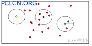
2)RadiusOutlierRemoval
它的原理是在点云数据中,用户指定每个的点一定范围内周围至少要有足够多的近邻。例如,如果指定至少要有1个邻居,只有黄色的点会被删除,如果指定至少要有2个邻居,黄色和绿色的点都将被删除。
(四):关键帧
一、整体介绍
在图优化中,关键帧的作用是不言而喻的,一个关键帧就对应一个顶点。在这个系统中,关键中对应的文件有两类:
src/hdl_graph_slam/keyframe.cpp 和include/hdl_graph_slam/keyframe.hpp
它包含KeyFrame和KeyFrameSnapshot两个类。
KeyFrame类对应的所有优化相关的信息,包括gps、imu等信息都在里面,另外它还有一个作用就是把这些信息存入文件,并在需要的时候从文件中读取这些信息,其实是为了离线优化。
KeyFrameSnapshot类可以理解为简化版的KeyFrame类,它只包含位姿和点云信息,是拼接地图时用的,因为一张地图只需要每一帧的位姿和原始点云就好了呀
- include/hdl_graph_slam/keyframe_updater.hpp
它包含KeyFramUpdater类,作用是更新关键帧,就是判断当前帧和上一个关键帧是否在距离或者角度上达到了一定差距,如果是,则把它设置为关键帧。
二、详细介绍
下面我们就进入这两个文件的内部,看一下到底做了啥
- KeyFrame类
它对应的代码在文件keyframe.cpp/.hpp中
1)包含的信息
从keyframe.hpp的代码中,我们可以清晰看出一个关键帧都包含了哪些信息
ros::Time stamp;                                // timestamp
  Eigen::Isometry3d odom;                         // odometry (estimated by scan_matching_odometry)
  double accum_distance;                          // accumulated distance from the first node (by scan_matching_odometry)
  pcl::PointCloud<PointT>::ConstPtr cloud;        // point cloud
  boost::optional<Eigen::Vector4d> floor_coeffs;  // detected floor's coefficients
  boost::optional<Eigen::Vector3d> utm_coord;     // UTM coord obtained by GPS

  boost::optional<Eigen::Vector3d> acceleration;   //
  boost::optional<Eigen::Quaterniond> orientation; //

  g2o::VertexSE3* node;                           // node instance
英文注释应该也都能看得懂,不解释了吧
2)读写信息
读和写分别对应save和load函数,内容简单明了,直接贴代码吧
void KeyFrame::save(const std::string& directory) {
  if(!boost::filesystem::is_directory(directory)) {
    boost::filesystem::create_directory(directory);
  }

  std::ofstream ofs(directory + "/data");
  ofs << "stamp " << stamp.sec << " " << stamp.nsec << "\n";

  ofs << "estimate\n";
  ofs << node->estimate().matrix() << "\n";

  ofs << "odom\n";
  ofs << odom.matrix() << "\n";

  ofs << "accum_distance " << accum_distance << "\n";

  if(floor_coeffs) {
    ofs << "floor_coeffs " << floor_coeffs->transpose() << "\n";
  }

  if(utm_coord) {
      ofs << "utm_coord " << utm_coord->transpose() << "\n";
  }

  if(acceleration) {
      ofs << "acceleration " << acceleration->transpose() << "\n";
  }

  if(orientation) {
      ofs << "orientation " << orientation->w() << " " << orientation->x() << " " << orientation->y() << " " << orientation->z() << "\n";
  }

  if(node) {
    ofs << "id " << node->id() << "\n";
  }

  pcl::io::savePCDFileBinary(directory + "/cloud.pcd", *cloud);
}

bool KeyFrame::load(const std::string& directory, g2o::HyperGraph* graph) {
    std::ifstream ifs(directory + "/data");
    if(!ifs) {
        return false;
    }

    long node_id = -1;
    boost::optional<Eigen::Isometry3d> estimate;

    while(!ifs.eof()) {
        std::string token;
        ifs >> token;

        if(token == "stamp") {
            ifs >> stamp.sec >> stamp.nsec;
        } else if(token == "estimate") {
            Eigen::Matrix4d mat;
            for(int i=0; i<4; i++) {
                for(int j=0; j<4; j++) {
                    ifs >> mat(i, j);
                }
            }
            estimate = Eigen::Isometry3d::Identity();
            estimate->linear() = mat.block<3, 3>(0, 0);
            estimate->translation() = mat.block<3, 1>(0, 3);
        } else if(token == "odom") {
            Eigen::Matrix4d odom_mat = Eigen::Matrix4d::Identity();
            for(int i=0; i<4; i++) {
                for(int j=0; j<4; j++) {
                    ifs >> odom_mat(i, j);
                }
            }

            odom.setIdentity();
            odom.linear() = odom_mat.block<3, 3>(0, 0);
            odom.translation() = odom_mat.block<3, 1>(0, 3);
        } else if(token == "accum_distance") {
            ifs >> accum_distance;
        } else if(token == "floor_coeffs") {
            Eigen::Vector4d coeffs;
            ifs >> coeffs[0] >> coeffs[1] >> coeffs[2] >> coeffs[3];
            floor_coeffs = coeffs;
        } else if (token == "utm_coord") {
            Eigen::Vector3d coord;
            ifs >> coord[0] >> coord[1] >> coord[2];
            utm_coord = coord;
        } else if(token == "acceleration") {
            Eigen::Vector3d acc;
            ifs >> acc[0] >> acc[1] >> acc[2];
            acceleration = acc;
        } else if(token == "orientation") {
            Eigen::Quaterniond quat;
            ifs >> quat.w() >> quat.x() >> quat.y() >> quat.z();
            orientation = quat;
        } else if(token == "id") {
            ifs >> node_id;
        }
    }

    if(node_id < 0) {
        ROS_ERROR_STREAM("invalid node id!!");
        ROS_ERROR_STREAM(directory);
        return false;
    }

    node = dynamic_cast<g2o::VertexSE3*>(graph->vertices()[node_id]);
    if(node == nullptr) {
        ROS_ERROR_STREAM("failed to downcast!!");
        return false;
    }

    if(estimate) {
        node->setEstimate(*estimate);
    }

    pcl::PointCloud<PointT>::Ptr cloud_(new pcl::PointCloud<PointT>());
    pcl::io::loadPCDFile(directory + "/cloud.pcd", *cloud_);
    cloud = cloud_;

    return true;
}
2. KeyFrameSnapshot类
它对应的代码同样在文件keyframe.cpp/.hpp中。

包含的信息如下,可以看到只有位姿和点云

Eigen::Isometry3d pose;                   // pose estimated by graph optimization
pcl::PointCloud<PointT>::ConstPtr cloud;
构造函数如下

KeyFrameSnapshot::KeyFrameSnapshot(const Eigen::Isometry3d& pose, const pcl::PointCloud<PointT>::ConstPtr& cloud)
  : pose(pose),
    cloud(cloud)
{}

KeyFrameSnapshot::KeyFrameSnapshot(const KeyFrame::Ptr& key)
  : pose(key->node->estimate()),
    cloud(key->cloud)
{}
从它的构造函数中可以看出,在实际使用时,它的内容都是从KeyFrame类中获得的,具体什么时候获得,怎样获得,我们后面会讲
- KeyFrameUpdater类
它在文件keyframe_updater.hpp中,它的作用和工作流程我们在上面已经介绍了,这些内容就放在一个update函数里,简单。
bool update(const Eigen::Isometry3d& pose) {
    // first frame is always registered to the graph
    if(is_first) {
      is_first = false;
      prev_keypose = pose;
      return true;
    }

    // calculate the delta transformation from the previous keyframe
    Eigen::Isometry3d delta = prev_keypose.inverse() * pose;
    double dx = delta.translation().norm();
    double da = std::acos(Eigen::Quaterniond(delta.linear()).w());

    // too close to the previous frame
    if(dx < keyframe_delta_trans && da < keyframe_delta_angle) {
      return false;
    }

    accum_distance += dx;
    prev_keypose = pose;
    return true;
  }
这个文件里包含的内容其实并不多,我认为把它独立成一个类的做法可有可无,会稍微清晰一些,但必要性也没有特别大。
(五):前端里程计
前端里程计的主要代码在apps/scan_matching_odometry_nodelet.cpp中,它的主要作用是订阅点云、匹配得到位姿,并以odom形式发布位姿。
对于订阅发布数据之类的,属于ros的基础内容,我们不在这里介绍了,我们介绍核心内容,即点云配准这部分。
点云匹配包括两方面内容,一是根据配置文件选择点云匹配方法,二是根据订阅得到的点云去匹配得到位姿。
我们把这两方面内容分别介绍。
- 选择匹配方法
这个函数在文件src/hdl_graph_slam/registrations.cpp中,我们看下代码
boost::shared_ptr<pcl::Registration<pcl::PointXYZI, pcl::PointXYZI>> select_registration_method(ros::NodeHandle& pnh) {
  using PointT = pcl::PointXYZI;

  // select a registration method (ICP, GICP, NDT)
  std::string registration_method = pnh.param<std::string>("registration_method", "NDT_OMP");
  if(registration_method == "ICP") {
    std::cout << "registration: ICP" << std::endl;
    boost::shared_ptr<pcl::IterativeClosestPoint<PointT, PointT>> icp(new pcl::IterativeClosestPoint<PointT, PointT>());
    icp->setTransformationEpsilon(pnh.param<double>("transformation_epsilon", 0.01));
    icp->setMaximumIterations(pnh.param<int>("maximum_iterations", 64));
    icp->setUseReciprocalCorrespondences(pnh.param<bool>("use_reciprocal_correspondences", false));
    return icp;
  } else if(registration_method.find("GICP") != std::string::npos) {
    if(registration_method.find("OMP") == std::string::npos) {
      std::cout << "registration: GICP" << std::endl;
      boost::shared_ptr<pcl::GeneralizedIterativeClosestPoint<PointT, PointT>> gicp(new pcl::GeneralizedIterativeClosestPoint<PointT, PointT>());
      gicp->setTransformationEpsilon(pnh.param<double>("transformation_epsilon", 0.01));
      gicp->setMaximumIterations(pnh.param<int>("maximum_iterations", 64));
      gicp->setUseReciprocalCorrespondences(pnh.param<bool>("use_reciprocal_correspondences", false));
      gicp->setCorrespondenceRandomness(pnh.param<int>("gicp_correspondence_randomness", 20));
      gicp->setMaximumOptimizerIterations(pnh.param<int>("gicp_max_optimizer_iterations", 20));
      return gicp;
    } else {
      std::cout << "registration: GICP_OMP" << std::endl;
      boost::shared_ptr<pclomp::GeneralizedIterativeClosestPoint<PointT, PointT>> gicp(new pclomp::GeneralizedIterativeClosestPoint<PointT, PointT>());
      gicp->setTransformationEpsilon(pnh.param<double>("transformation_epsilon", 0.01));
      gicp->setMaximumIterations(pnh.param<int>("maximum_iterations", 64));
      gicp->setUseReciprocalCorrespondences(pnh.param<bool>("use_reciprocal_correspondences", false));
      gicp->setCorrespondenceRandomness(pnh.param<int>("gicp_correspondence_randomness", 20));
      gicp->setMaximumOptimizerIterations(pnh.param<int>("gicp_max_optimizer_iterations", 20));
      return gicp;
    }
  } else {
    if(registration_method.find("NDT") == std::string::npos ) {
      std::cerr << "warning: unknown registration type(" << registration_method << ")" << std::endl;
      std::cerr << "       : use NDT" << std::endl;
    }

    double ndt_resolution = pnh.param<double>("ndt_resolution", 0.5);
    if(registration_method.find("OMP") == std::string::npos) {
      std::cout << "registration: NDT " << ndt_resolution << std::endl;
      boost::shared_ptr<pcl::NormalDistributionsTransform<PointT, PointT>> ndt(new pcl::NormalDistributionsTransform<PointT, PointT>());
      ndt->setTransformationEpsilon(pnh.param<double>("transformation_epsilon", 0.01));
      ndt->setMaximumIterations(pnh.param<int>("maximum_iterations", 64));
      ndt->setResolution(ndt_resolution);
      return ndt;
    } else {
      int num_threads = pnh.param<int>("ndt_num_threads", 0);
      std::string nn_search_method = pnh.param<std::string>("ndt_nn_search_method", "DIRECT7");
      std::cout << "registration: NDT_OMP " << nn_search_method << " " << ndt_resolution << " (" << num_threads << " threads)" << std::endl;
      boost::shared_ptr<pclomp::NormalDistributionsTransform<PointT, PointT>> ndt(new pclomp::NormalDistributionsTransform<PointT, PointT>());
      if(num_threads > 0) {
        ndt->setNumThreads(num_threads);
      }
      ndt->setTransformationEpsilon(pnh.param<double>("transformation_epsilon", 0.01));
      ndt->setMaximumIterations(pnh.param<int>("maximum_iterations", 64));
      ndt->setResolution(ndt_resolution);
      if(nn_search_method == "KDTREE") {
        ndt->setNeighborhoodSearchMethod(pclomp::KDTREE);
      } else if (nn_search_method == "DIRECT1") {
        ndt->setNeighborhoodSearchMethod(pclomp::DIRECT1);
      } else {
        ndt->setNeighborhoodSearchMethod(pclomp::DIRECT7);
      }
      return ndt;
    }
  }

  return nullptr;
}
别看代码这么长,其实流程很简单,就是根据从配置文件读取的registration_method这个配置项来选择相应的匹配算法,选择匹配算法以后再把这个算法对应的参数从配置文件中读取出来即可。
可选择的匹配算法一共包括:ICP、GICP、GICP_OMP、NDT、NDT_OMP,这里ICP、GICP和NDT都是经典的点云配准方法,感兴趣的可以自己去网上查资料,而带OMP字样的两种方法,指的是对应方法的多线程版本,可以缩短匹配算法的执行时间。
最后说以下返回值,这个函数的返回类型是boost::shared_ptr<pcl::Registration<pcl::PointXYZI, pcl::PointXYZI>>,以上提到的所有方法都是pcl库下面的,而pcl::Registration就是所有这些方法的基类,都继承自它,所以不管选择了什么方法,都可以返回该方法的指针。
- 点云匹配
点云匹配的代码在apps/scan_matching_odometry_nodelet.cpp中,其实就是对应一个matching函数,它的代码如下
Eigen::Matrix4f matching(const ros::Time& stamp, const pcl::PointCloud::ConstPtr& cloud) {
//还没有关键帧,说明它是第一帧,则直接把它设置成关键帧,并初始化位姿为单位阵,直接返回
if(!keyframe) {
prev_trans.setIdentity();
keyframe_pose.setIdentity();
keyframe_stamp = stamp;
keyframe = downsample(cloud);
registration->setInputTarget(keyframe);
return Eigen::Matrix4f::Identity();
}
//当前点云给registration
auto filtered = downsample(cloud);
registration->setInputSource(filtered);
//执行匹配
pcl::PointCloud::Ptr aligned(new pcl::PointCloud());
registration->align(*aligned, prev_trans);
//匹配结束,则返回它相对于关键帧额位姿
if(!registration->hasConverged()) {
NODELET_INFO_STREAM(“scan matching has not converged!!”);
NODELET_INFO_STREAM(“ignore this frame(” << stamp << “)”);
return keyframe_pose * prev_trans;
}
Eigen::Matrix4f trans = registration->getFinalTransformation();
Eigen::Matrix4f odom = keyframe_pose * trans;

//这段代码的主要功能是判断当前匹配的相对位姿是否过大,载体不可能短时间内有这么大的运动
//所以如果出现了,就说明这一帧匹配可能不正常,则直接舍弃
if(transform_thresholding) {
  Eigen::Matrix4f delta = prev_trans.inverse() * trans;
  double dx = delta.block<3, 1>(0, 3).norm();
  double da = std::acos(Eigen::Quaternionf(delta.block<3, 3>(0, 0)).w());

  if(dx > max_acceptable_trans || da > max_acceptable_angle) {
    NODELET_INFO_STREAM("too large transform!!  " << dx << "[m] " << da << "[rad]");
    NODELET_INFO_STREAM("ignore this frame(" << stamp << ")");
    return keyframe_pose * prev_trans;
  }
}

prev_trans = trans;


auto keyframe_trans = matrix2transform(stamp, keyframe_pose, odom_frame_id, "keyframe");
keyframe_broadcaster.sendTransform(keyframe_trans);

//判断这一帧相对于关键帧的位置或角度是否比较大了
//如果比较大,则需要更新关键帧,并把新的关键帧的点云设置成Target
double delta_trans = trans.block<3, 1>(0, 3).norm();
double delta_angle = std::acos(Eigen::Quaternionf(trans.block<3, 3>(0, 0)).w());
double delta_time = (stamp - keyframe_stamp).toSec();
if(delta_trans > keyframe_delta_trans || delta_angle > keyframe_delta_angle || delta_time > keyframe_delta_time) {
  keyframe = filtered;
  registration->setInputTarget(keyframe);

  keyframe_pose = odom;
  keyframe_stamp = stamp;
  prev_trans.setIdentity();
}

return odom;
}
点云匹配的流程比较清晰,我已经在代码里加了注释了,直接看注释应该就能看明白。
- 一点思考
它的这个匹配流程里面有优点也有缺点,优点是对当前的位姿做了异常判断,如果不合理,则舍弃这一帧,缺点是target只是当前关键帧,一帧点云作为target还是略显稀疏了,一般都有map的概念,这个map可以是一个滑窗,即相邻的几个关键帧共同组成一个target,这是常见的做法。它的前端里程计的效果并不好,这是一个重要的原因。
另一点就是在前端里程计中,包含了点云滤波和关键帧计算这两部分代码,滤波部分和之前介绍点云滤波的那一节里提到的prefiltering_nodelet.cpp文件中的代码完全一样,而关键帧计算部分的代码和之前在关键帧那一节里所提到的keyframe_updater.hpp的代码功能也一样,不清楚作者为啥把同样的东西写两遍,这明显是重复代码,至少从代码规范上不合理。
(六):地面检测
地面检测的作用我们在第一节就讲过了,它为建图提供一个约束,可以提高建图精度。
地面检测的代码全都在apps/floor_detection_nodelet.cpp文件中,这是一个节点文件,里面关于订阅和发布数据的内容我们不讲了,只介绍关于检测的核心算法。
地面检测共分为三个步骤:
1)根据高度参数把地面分割出来,由函数plane_clip完成
2)把地面点云中,去掉法向量和地面实际法向量差别较大的点,这一步由函数normal_filtering完成
3)对剩下的点进行平面参数拟合,这部分代码在函数detect中(前两部对应的函数也是在detect中被调用)
下面我们就对这三部分内容分别介绍
1. 分割地面
思路比较简单,由于pcl::PlaneClipper3D可以把指定点云区域一侧的点全部去掉,所以执行两次滤波就可以了,两次分别把地面高度上面和下面的点全部去掉,就只剩下地面点云了。
先看plane_clip函数,也就是去掉一侧点云的函数,没太多可讲的,pcl函数调用的标准流程,给它参数,然后执行就可以了。
pcl::PointCloud::Ptr plane_clip(const pcl::PointCloud::Ptr& src_cloud, const Eigen::Vector4f& plane, bool negative) const {
pcl::PlaneClipper3D clipper(plane);
pcl::PointIndices::Ptr indices(new pcl::PointIndices);
clipper.clipPointCloud3D(*src_cloud, indices->indices);

pcl::PointCloud<PointT>::Ptr dst_cloud(new pcl::PointCloud<PointT>);

pcl::ExtractIndices<PointT> extract;
extract.setInputCloud(src_cloud);
extract.setIndices(indices);
extract.setNegative(negative);
extract.filter(*dst_cloud);

return dst_cloud;
}
然后这个函数在detect函数中被调用了两次
pcl::PointCloud::Ptr filtered(new pcl::PointCloud);
pcl::transformPointCloud(*cloud, *filtered, tilt_matrix);
filtered = plane_clip(filtered, Eigen::Vector4f(0.0f, 0.0f, 1.0f, sensor_height + height_clip_range), false);
filtered = plane_clip(filtered, Eigen::Vector4f(0.0f, 0.0f, 1.0f, sensor_height - height_clip_range), true);
这两次就把地面上下两个方向的其他点云都去掉了
2. 去掉法向量异常的点
地面点云每个点所处位置对应的法向量都应该是向上的,即使有些差异,也不应该过大,否则就不是地面点,按照这个思路,我们又可以去掉一部分点云。这里法向量计算是用的pcl库中的函数pcl::NormalEstimation
pcl::PointCloud::Ptr normal_filtering(const pcl::PointCloud::Ptr& cloud) const {
pcl::NormalEstimation<PointT, pcl::Normal> ne;
ne.setInputCloud(cloud);
    pcl::search::KdTree<PointT>::Ptr tree(new pcl::search::KdTree<PointT>);
    ne.setSearchMethod(tree);

    pcl::PointCloud<pcl::Normal>::Ptr normals(new pcl::PointCloud<pcl::Normal>);
    ne.setKSearch(10);
    ne.setViewPoint(0.0f, 0.0f, sensor_height);
    ne.compute(*normals);//计算地面点云的法向量

    pcl::PointCloud<PointT>::Ptr filtered(new pcl::PointCloud<PointT>);
    filtered->reserve(cloud->size());
    //这段是核心,遍历所有的点,法向量满足要求时这个点才被选取
    for (int i = 0; i < cloud->size(); i++) {
      float dot = normals->at(i).getNormalVector3fMap().normalized().dot(Eigen::Vector3f::UnitZ());
      if (std::abs(dot) > std::cos(normal_filter_thresh * M_PI / 180.0)) {
        filtered->push_back(cloud->at(i));
      }
    }

    filtered->width = filtered->size();
    filtered->height = 1;
    filtered->is_dense = false;

    return filtered;
  }
3. 拟合平面参数
现在我们有了一个平面对应的点云,需要对他进行拟合。这部分代码来自detect函数,拟合所用的算法也是使用pcl库
//点太少,则直接退出
if(filtered->size() < floor_pts_thresh) {
  return boost::none;
}

// RANSAC
pcl::SampleConsensusModelPlane<PointT>::Ptr model_p(new pcl::SampleConsensusModelPlane<PointT>(filtered));
pcl::RandomSampleConsensus<PointT> ransac(model_p);
ransac.setDistanceThreshold(0.1);
ransac.computeModel();

pcl::PointIndices::Ptr inliers(new pcl::PointIndices);
ransac.getInliers(inliers->indices);

// too few inliers
//内点过少,也退出
if(inliers->indices.size() < floor_pts_thresh) {
  return boost::none;
}

// verticality check of the detected floor's normal
Eigen::Vector4f reference = tilt_matrix.inverse() * Eigen::Vector4f::UnitZ();

Eigen::VectorXf coeffs;
ransac.getModelCoefficients(coeffs);

double dot = coeffs.head<3>().dot(reference.head<3>());
//法向量不合理,退出
if(std::abs(dot) < std::cos(floor_normal_thresh * M_PI / 180.0)) {
  // the normal is not vertical
  return boost::none;
}

// make the normal upward
// 法向量颠倒个方向
if(coeffs.head<3>().dot(Eigen::Vector3f::UnitZ()) < 0.0f) {
  coeffs *= -1.0f;
}
(七):闭环检测
做slam怎么能少得了闭环。
闭环检测的代码在文件include/hdl_graph_slam/loop_detector.hpp中,整个流程分布的很清晰,我们直接进入看代码的环节了
1. 整体流程
在调用闭环检测功能时,实际是调用的函数detect,所以我们直接看这个函数,就可以看出它的流程
std::vectorLoop::Ptr detect(const std::vectorKeyFrame::Ptr& keyframes, const std::dequeKeyFrame::Ptr& new_keyframes, hdl_graph_slam::GraphSLAM& graph_slam) {
std::vectorLoop::Ptr detected_loops;
for(const auto& new_keyframe : new_keyframes) {
auto candidates = find_candidates(keyframes, new_keyframe);
auto loop = matching(candidates, new_keyframe, graph_slam);
if(loop) {
detected_loops.push_back(loop);
}
}
return detected_loops;
}
它的输入是:
1)keyframes:已有的关键帧
2)new_keyframes:新增的关键帧
3)graph_slam:这个参数没有被用到,估计作者可能是原计划要用,但后来没用到,也忘了删了
它的输出是:
1)std::vectorLoop::Ptr:所有检测成功的匹配关系
具体来讲,包括它是由哪两帧匹配的,匹配计算得到的相对位姿是多少。
这个看Loop这个结构提的定义就明白了
struct Loop {
public:
EIGEN_MAKE_ALIGNED_OPERATOR_NEW
using Ptr = std::shared_ptr;
-
Loop(const KeyFrame::Ptr& key1, const KeyFrame::Ptr& key2, const Eigen::Matrix4f& relpose)
-
key1(key1),
key2(key2),
relative_pose(relpose)
{}
public:
KeyFrame::Ptr key1;
KeyFrame::Ptr key2;
Eigen::Matrix4f relative_pose;
};
它包含的就是上面我们所提到的这三个信息。
由于每次检测可能有多个新增的关键帧要参与,有可能检测到多对匹配关系,所以这里用一个vector把所有关系同时输出。
弄明白输入输出,这个函数的功能就可以概括了:
从已有的关键帧中,检测与新增的关键帧是否有闭环关系,如果有,则返回所有检测结果。
而且上面的代码还告诉了我们)进行闭环检测的步骤:
1)检测满足条件的关键帧,以进行下一步匹配
2)对检测到的关键帧进行匹配,找出匹配精度最好的一帧,并返回匹配关系
3)把第2)步找到的匹配关系放入容器中
4)循环上面三步,直到所有新的关键帧遍历完
上面四步中,第3)和第4)部就是几行语句而已,需要展开介绍的是第1)和第2)步,下面我们就分别对这两步进行介绍。
2. 检测满足条件的关键帧
这个功能被封装在了函数find_candidates中,我们看它的代码
std::vectorKeyFrame::Ptr find_candidates(const std::vectorKeyFrame::Ptr& keyframes, const KeyFrame::Ptr& new_keyframe) const {
// too close to the last registered loop edge
if(new_keyframe->accum_distance - last_edge_accum_distance < distance_from_last_edge_thresh) {
return std::vectorKeyFrame::Ptr();
}
std::vector<KeyFrame::Ptr> candidates;
candidates.reserve(32);

for(const auto& k : keyframes) {
  // traveled distance between keyframes is too small
  if(new_keyframe->accum_distance - k->accum_distance < accum_distance_thresh) {
    continue;
  }

  const auto& pos1 = k->node->estimate().translation();
  const auto& pos2 = new_keyframe->node->estimate().translation();

  // estimated distance between keyframes is too small
  double dist = (pos1.head<2>() - pos2.head<2>()).norm();
  if(dist > distance_thresh) {
    continue;
  }

  candidates.push_back(k);
}

return candidates;
}
从上面的代码中我们可以看到,所谓的满足条件,指的是满足以下条件:
1)新的关键帧离上一个被闭环的帧“里程距离”不能过小
注意,这里特意强调了是“里程距离”,我们举个例子,来弄明白这个概念。
比如第1帧往前走了1米得到了第2帧,第2帧往后走了1米得到了第3帧,那么第1帧和第3帧的“直线距离”就是0,但是总的里程是2米,所以他们的“里程距离”就是2。闭环应该找“直线距离”尽量进而“里程距离”尽量远的,所以这里才要求“里程距离”不能过小。
其实我觉得给每一个关键帧一个编号,编号顺序递增,用编号计算一个“编号距离”应该更简单,不用每次还要计算“里程距离”这么麻烦。
弄明白了它的原理,我们就清楚它的作用了,就是把闭环关系弄的稀疏一些,别整那么多,如果来了是个关键帧,没一帧都弄了一个闭环边添加到图里,也没那个必要,所以有了这一步以后,我们会在所有新的关键帧中取一小部分建立闭环关系,既能起到约束作用,又不至于把模型弄的复杂。
2)已有关键帧离新的关键帧的“里程距离”不能过小
3)已有关键帧和新的关键帧之间的“直线距离”要足够小
能够同时满足这三个条件的就可以进入下一步的匹配环节了。
3. 闭环匹配
上一步索引出来的关键帧还要通过这一步的检验,才能够算是真正成功实现了闭环匹配。这一步在函数matching中,我们还是直接看代码
Loop::Ptr matching(const std::vectorKeyFrame::Ptr& candidate_keyframes, const KeyFrame::Ptr& new_keyframe, hdl_graph_slam::GraphSLAM& graph_slam) {
if(candidate_keyframes.empty()) {
return nullptr;
}
registration->setInputTarget(new_keyframe->cloud);

double best_score = std::numeric_limits<double>::max();
KeyFrame::Ptr best_matched;
Eigen::Matrix4f relative_pose;

std::cout << std::endl;
std::cout << "--- loop detection ---" << std::endl;
std::cout << "num_candidates: " << candidate_keyframes.size() << std::endl;
std::cout << "matching" << std::flush;
auto t1 = ros::Time::now();

pcl::PointCloud<PointT>::Ptr aligned(new pcl::PointCloud<PointT>());
for(const auto& candidate : candidate_keyframes) {
  registration->setInputSource(candidate->cloud);
  Eigen::Matrix4f guess = (new_keyframe->node->estimate().inverse() * candidate->node->estimate()).matrix().cast<float>();
  guess(2, 3) = 0.0;
  registration->align(*aligned, guess);
  std::cout << "." << std::flush;

  double score = registration->getFitnessScore(fitness_score_max_range);
  if(!registration->hasConverged() || score > best_score) {
    continue;
  }

  best_score = score;
  best_matched = candidate;
  relative_pose = registration->getFinalTransformation();
}

auto t2 = ros::Time::now();
std::cout << " done" << std::endl;
std::cout << "best_score: " << boost::format("%.3f") % best_score << "    time: " << boost::format("%.3f") % (t2 - t1).toSec() << "[sec]" << std::endl;

if(best_score > fitness_score_thresh) {
  std::cout << "loop not found..." << std::endl;
  return nullptr;
}

std::cout << "loop found!!" << std::endl;
std::cout << "relpose: " << relative_pose.block<3, 1>(0, 3) << " - " << Eigen::Quaternionf(relative_pose.block<3, 3>(0, 0)).coeffs().transpose() << std::endl;

last_edge_accum_distance = new_keyframe->accum_distance;

return std::make_shared<Loop>(new_keyframe, best_matched, relative_pose);
}
从上面的代码中我们可以看到,它的核心流程可以概括如下:
1)对每一个关键帧都和新帧进行点云匹配,看匹配精度满足闭环的基本要求
2)如果满足,则在所有满足条件的关键帧中找出匹配精度最高的那一帧
4. 一点思考
在上面的流程中,我认为还是有一些不合理的地方
1)匹配点云的时候还是只对两帧进行匹配,这一点我们在讲前端里程计的时候就提到过,我认为把关键帧的前后几帧都找出来,拼成一个局部地图再去匹配应该精度会更高,毕竟两帧点云匹配太稀疏了。
2)对所有满足条件的关键帧都做一次点云匹配太浪费时间了,帧间匹配还是挺耗时间的,当地图稍微大一些,有几千个关键帧的时候,一个闭环检测要匹配多少次,这肯定不行。我认为找一个距离最近的关键帧,然后以它为中心取前后几帧构建一个局部地图去匹配就行了,精度满足就建一条闭环边,不满足就不要了,等下一次。
(八):后端优化
一、整体介绍
这部分是整个系统的核心,因为这个系统就是建图的呀,建图的核心就是综合所有信息进行优化呀。我们前面几节介绍的所有的信息都会发送到这个节点中来供它使用。这部分的代码在文件apps/hdl_graph_slam_nodelet.cpp中。
这部分的代码看着挺多,如果我们能够对它所有的函数分类,就很容易梳理它的内容了。
我们刚才提到,它需要接收之前几节介绍的所有的信息,并加入概率图中,所以我们以信息为切入点,去梳理它的内容。
我们先看都包含哪些信息:
1)前端里程计传入的位姿和点云
2)gps信息
3)Imu信息
4)平面拟合的参数信息
处理一个信息包括以下步骤:
1)在对应的callback函数中接收信息,并放入相应的队列
2)根据时间戳对队列中的信息进行顺序处理,加入概率图
四条信息,每条信息都执行两个步骤,这就已经包含了本文件大部分的代码。
剩下的就是一些其他内容,我们进一步梳理:
1)执行图优化,这是一个定时执行的函数,闭环检测也在这个函数里
2)生成全局地图并定时发送,即把所有关键帧拼一起,得到全局点云地图,然后在一个定时函数里发送到rviz上去
3)在rviz中显示顶点和边,如果运行程序,会看到rviz中把概率图可视化了
至此,整个文件的核心框ros架就梳理完了,剩下的一些细枝末节的东西应该都能看懂。
下面我们就按照这个框架对各部分内容进行梳理,这次梳理我们遵照以下原则:
1)和消息相关的代码我们之前在各自对应的章节中都梳理过了,这里只是使用,所以他们的代码就不贴出来了,不然会把本节内容搞得繁琐,反而不利于整体理解
2)概率图可视化的代码就不解释了,和核心算法无关
3)和算法无关的一些ros操作相关的东西,也不在这里解释了
二、代码详解
- 前端里程计消息处理
还记得那两个步骤吗?
1)接收消息:cloud_callback
2)处理消息队列:flush_keyframe_queue
- gps消息
1)接收消息:nmea_callback + navsat_callback + gps_callback
2)处理消息队列:flush_gps_queue
- imu消息
1)接收消息:imu_callback
2)处理消息队列:flush_imu_queue
- 地面拟合参数
1)接收消息:floor_coeffs_callback
2)处理消息队列:flush_floor_queue
- 执行图优化
函数名是optimization_timer_callback,这个函数除了执行图优化意外,还做了以下两点:
1)闭环检测
// loop detection
    std::vector<Loop::Ptr> loops = loop_detector->detect(keyframes, new_keyframes, *graph_slam);
    for(const auto& loop : loops) {
      Eigen::Isometry3d relpose(loop->relative_pose.cast<double>());
      Eigen::MatrixXd information_matrix = inf_calclator->calc_information_matrix(loop->key1->cloud, loop->key2->cloud, relpose);
      auto edge = graph_slam->add_se3_edge(loop->key1->node, loop->key2->node, relpose, information_matrix);
      graph_slam->add_robust_kernel(edge, private_nh.param<std::string>("loop_closure_edge_robust_kernel", "NONE"), private_nh.param<double>("loop_closure_edge_robust_kernel_size", 1.0));
    }
检测闭环并加到了概率图中,当然实在优化之前
2)生成简化版关键帧
还记得我们在关键帧那一节介绍的简化版关键帧(KeyFrameSnapshot)吗?
它从KeyFrame类中取出位姿(当然是优化之后的位姿)和点云,供地图拼接使用,这样我们得到的就是位姿经过优化的地图了。
std::vector<KeyFrameSnapshot::Ptr> snapshot(keyframes.size());
    std::transform(keyframes.begin(), keyframes.end(), snapshot.begin(),
      [=](const KeyFrame::Ptr& k) {
        return std::make_shared<KeyFrameSnapshot>(k);
    });

    keyframes_snapshot_mutex.lock();
    keyframes_snapshot.swap(snapshot);
    keyframes_snapshot_mutex.unlock();
- 生成地图并定时发送
生成地图并定时发送很明显包括两步:生成地图、定时发送,哈哈
1)生成地图
就是使用简化版关键帧进行拼接,这部分代码在文件src/hdl_graph_slam/map_cloud_generator.cpp中,更具体点说,就是里面的generate函数,其实就是个拼接的过程。
pcl::PointCloud<MapCloudGenerator::PointT>::Ptr MapCloudGenerator::generate(const std::vector<KeyFrameSnapshot::Ptr>& keyframes, double resolution) const {
  if(keyframes.empty()) {
    std::cerr << "warning: keyframes empty!!" << std::endl;
    return nullptr;
  }

  pcl::PointCloud<PointT>::Ptr cloud(new pcl::PointCloud<PointT>());
  cloud->reserve(keyframes.front()->cloud->size() * keyframes.size());

  for(const auto& keyframe : keyframes) {
    Eigen::Matrix4f pose = keyframe->pose.matrix().cast<float>();
    for(const auto& src_pt : keyframe->cloud->points) {
      PointT dst_pt;
      dst_pt.getVector4fMap() = pose * src_pt.getVector4fMap();
      dst_pt.intensity = src_pt.intensity;
      cloud->push_back(dst_pt);
    }
  }

  cloud->width = cloud->size();
  cloud->height = 1;
  cloud->is_dense = false;

  pcl::octree::OctreePointCloud<PointT> octree(resolution);
  octree.setInputCloud(cloud);
  octree.addPointsFromInputCloud();

  pcl::PointCloud<PointT>::Ptr filtered(new pcl::PointCloud<PointT>());
  octree.getOccupiedVoxelCenters(filtered->points);

  filtered->width = filtered->size();
  filtered->height = 1;
  filtered->is_dense = false;

  return filtered;
}
2)定时发送
这部分内容在apps/hdl_graph_slam_nodelet.cpp文件中,简单,不解释了
void map_points_publish_timer_callback(const ros::WallTimerEvent& event) {
    if(!map_points_pub.getNumSubscribers()) {
      return;
    }

    std::vector<KeyFrameSnapshot::Ptr> snapshot;

    keyframes_snapshot_mutex.lock();
    snapshot = keyframes_snapshot;
    keyframes_snapshot_mutex.unlock();

    auto cloud = map_cloud_generator->generate(snapshot, 0.05);
    if(!cloud) {
      return;
    }

    cloud->header.frame_id = map_frame_id;
    cloud->header.stamp = snapshot.back()->cloud->header.stamp;

    sensor_msgs::PointCloud2Ptr cloud_msg(new sensor_msgs::PointCloud2());
    pcl::toROSMsg(*cloud, *cloud_msg);

    map_points_pub.publish(cloud_msg);
  }
===分割线=
OK,整个hdl_graph_slam系统的介绍到这里就结束了,前后一共八篇文章。最后总结一下吧,虽然hdl_graph_slam的性能其实不是很好,具体原因在于帧间匹配和闭环检测的精度都不够,它在这两个环节的缺点我们在对应的章节已经解释过了。但是,但是,但是,我想说的是对于一套开源系统来讲,不能指望它拿来即用,小的缺点很容易改,都已经指出问题了,就那几行代码,改一改还不容易吗。我们更应该关心它的架构,这套系统的代码模块画做的很好,思路很清晰,整个系统对于对多信息源的融合做的很好,按照这种架构,再多来几个传感器也没关系,这就是系统的扩展性。综上,我认为对开发者来讲(注意这句话),这是一套不错的开源系统。


 412
412


 被折叠的 条评论
为什么被折叠?
被折叠的 条评论
为什么被折叠?
 到【灌水乐园】发言


