PyG (PyTorch Geometric) GNN 笔记

https://pytorch-geometric.readthedocs.io/en/latest/index.html

INTRODUCTION BY EXAMPLE

https://pytorch-geometric.readthedocs.io/en/latest/notes/introduction.html

A graph is used to model pairwise relations (edges) between objects (nodes). A single graph in PyG is described by an instance of torch_geometric.data.Data, which holds the following attributes by default:

data.x: Node feature matrix with shape [num_nodes, num_node_features] 节点特征矩阵
data.edge_index: Graph connectivity in COO format with shape [2, num_edges] and type torch.long 图连通性
data.edge_attr: Edge feature matrix with shape [num_edges, num_edge_features]
data.y: Target to train against (may have arbitrary shape), e.g., node-level targets of shape [num_nodes, *] or graph-level targets of shape [1, *]
data.pos: Node position matrix with shape [num_nodes, num_dimensions]

#After learning about data handling, datasets, loader and transforms in PyG, it’s time to implement our first graph neural network!

#We will use a simple GCN layer and replicate the experiments on the Cora citation dataset.
# For a high-level explanation on GCN, have a look at its blog post.

#We first need to load the Cora dataset:
from torch_geometric.datasets import Planetoid
dataset = Planetoid(root='/tmp/Cora', name='Cora')
>>> Cora()

#Note that we do not need to use transforms or a dataloader. Now let’s implement a two-layer GCN:
import torch
import torch.nn.functional as F
from torch_geometric.nn import GCNConv
class GCN(torch.nn.Module):
    def __init__(self):
        super().__init__()
        self.conv1 = GCNConv(dataset.num_node_features, 16)
        self.conv2 = GCNConv(16, dataset.num_classes)

    def forward(self, data):
        x, edge_index = data.x, data.edge_index
        x = self.conv1(x, edge_index)
        x = F.relu(x)
        x = F.dropout(x, training=self.training)
        x = self.conv2(x, edge_index)

        return F.log_softmax(x, dim=1)

#The constructor defines two GCNConv layers which get called in the forward pass of our network. 
#Note that the non-linearity is not integrated in the conv calls and hence needs to be applied afterwards (something which is consistent accross all operators in PyG). 
#Here, we chose to use ReLU as our intermediate non-linearity and finally output a softmax distribution over the number of classes. 
#Let’s train this model on the training nodes for 200 epochs:
device = torch.device('cuda' if torch.cuda.is_available() else 'cpu')
model = GCN().to(device)
data = dataset[0].to(device)
optimizer = torch.optim.Adam(model.parameters(), lr=0.01, weight_decay=5e-4)

model.train()
for epoch in range(200):
    optimizer.zero_grad()
    out = model(data)
    loss = F.nll_loss(out[data.train_mask], data.y[data.train_mask])
    loss.backward()
    optimizer.step()

#Finally, we can evaluate our model on the test nodes:
model.eval()
pred = model(data).argmax(dim=1)
correct = (pred[data.test_mask] == data.y[data.test_mask]).sum()
acc = int(correct) / int(data.test_mask.sum())
print(f'Accuracy: {acc:.4f}')
>>> Accuracy: 0.8150
#This is all it takes to implement your first graph neural network. 
#The easiest way to learn more about Graph Neural Networks is to study the examples in the examples/ directory and to browse torch_geometric.nn. 

COLAB NOTEBOOKS AND VIDEO TUTORIALS

https://pytorch-geometric.readthedocs.io/en/latest/notes/colabs.html?highlight=graph%20classification#colab-notebooks-and-video-tutorials

Graph Classification with Graph Neural Networks
https://colab.research.google.com/drive/1I8a0DfQ3fI7Njc62__mVXUlcAleUclnb?usp=sharing#scrollTo=N-FO5xL3mw98

# Install required packages.
!pip install -q torch-scatter -f https://pytorch-geometric.com/whl/torch-1.10.0+cu113.html
!pip install -q torch-sparse -f https://pytorch-geometric.com/whl/torch-1.10.0+cu113.html
!pip install -q git+https://github.com/rusty1s/pytorch_geometric.git

Graph Classification with Graph Neural Networks

The most common task for graph classification is molecular property prediction（分子特性预测）, in which molecules are represented as graphs, and the task may be to infer whether a molecule inhibits HIV virus replication or not.

The TU Dortmund University has collected a wide range of different graph classification datasets, known as the TUDatasets, which are also accessible via torch_geometric.datasets.TUDataset in PyTorch Geometric. Let’s load and inspect one of the smaller ones, the MUTAG dataset:

import torch
from torch_geometric.datasets import TUDataset

dataset = TUDataset(root='data/TUDataset', name='MUTAG')

print()
print(f'Dataset: {dataset}:')
print('====================')
print(f'Number of graphs: {len(dataset)}')
print(f'Number of features: {dataset.num_features}')
print(f'Number of classes: {dataset.num_classes}')

data = dataset[0]  # Get the first graph object.

print()
print(data)
print('=============================================================')

# Gather some statistics about the first graph.
print(f'Number of nodes: {data.num_nodes}')
print(f'Number of edges: {data.num_edges}')
print(f'Average node degree: {data.num_edges / data.num_nodes:.2f}')
print(f'Has isolated nodes: {data.has_isolated_nodes()}')
print(f'Has self-loops: {data.has_self_loops()}')
print(f'Is undirected: {data.is_undirected()}')

This dataset provides 188 different graphs, and the task is to classify each graph into one out of two classes.

By inspecting the first graph object of the dataset, we can see that it comes with 17 nodes (with 7-dimensional feature vectors) and 38 edges (leading to an average node degree of 2.24). It also comes with exactly one graph label (y=[1]), and, in addition to previous datasets, provides addtional 4-dimensional edge features (edge_attr=[38, 4]). However, for the sake of simplicity, we will not make use of those.

PyTorch Geometric provides some useful utilities for working with graph datasets, e.g., we can shuffle the dataset and use the first 150 graphs as training graphs, while using the remaining ones for testing:

torch.manual_seed(12345)
dataset = dataset.shuffle()

train_dataset = dataset[:150]
test_dataset = dataset[150:]

print(f'Number of training graphs: {len(train_dataset)}')
print(f'Number of test graphs: {len(test_dataset)}')

Mini-batching of graphs

Since graphs in graph classification datasets are usually small, a good idea is to batch the graphs before inputting them into a Graph Neural Network to guarantee full GPU utilization. In the image or language domain, this procedure is typically achieved by rescaling or padding each example into a set of equally-sized shapes, and examples are then grouped in an additional dimension. The length of this dimension is then equal to the number of examples grouped in a mini-batch and is typically referred to as the batch_size.

However, for GNNs the two approaches described above are either not feasible or may result in a lot of unnecessary memory consumption. Therefore, PyTorch Geometric opts for another approach to achieve parallelization across a number of examples. Here, adjacency matrices are stacked in a diagonal fashion (creating a giant graph that holds multiple isolated subgraphs), and node and target features are simply concatenated in the node dimension:

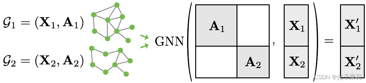
This procedure has some crucial advantages over other batching procedures:

GNN operators that rely on a message passing scheme do not need to be modified since messages are not exchanged between two nodes that belong to different graphs.

There is no computational or memory overhead since adjacency matrices are saved in a sparse fashion holding only non-zero entries, i.e., the edges.

PyTorch Geometric automatically takes care of batching multiple graphs into a single giant graph with the help of the torch_geometric.data.DataLoader class:

from torch_geometric.loader import DataLoader

train_loader = DataLoader(train_dataset, batch_size=64, shuffle=True)
test_loader = DataLoader(test_dataset, batch_size=64, shuffle=False)

for step, data in enumerate(train_loader):
    print(f'Step {step + 1}:')
    print('=======')
    print(f'Number of graphs in the current batch: {data.num_graphs}')
    print(data)
    print()

Here, we opt for a batch_size of 64, leading to 3 (randomly shuffled) mini-batches, containing all 2⋅64+22=150 graphs.

Furthermore, each Batch object is equipped with a batch vector, which maps each node to its respective graph in the batch:

batch=[0,…,0,1,…,1,2,…]

Training a Graph Neural Network (GNN)

Training a GNN for graph classification usually follows a simple recipe:

Embed each node by performing multiple rounds of message passing
Aggregate node embeddings into a unified graph embedding (readout layer)
Train a final classifier on the graph embedding
There exists multiple readout layers in literature, but the most common one is to simply take the average of node embeddings:

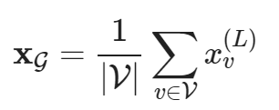
PyTorch Geometric provides this functionality via torch_geometric.nn.global_mean_pool, which takes in the node embeddings of all nodes in the mini-batch and the assignment vector batch to compute a graph embedding of size [batch_size, hidden_channels] for each graph in the batch.

The final architecture for applying GNNs to the task of graph classification then looks as follows and allows for complete end-to-end training:

from torch.nn import Linear
import torch.nn.functional as F
from torch_geometric.nn import GCNConv
from torch_geometric.nn import global_mean_pool


class GCN(torch.nn.Module):
    def __init__(self, hidden_channels):
        super(GCN, self).__init__()
        torch.manual_seed(12345)
        self.conv1 = GCNConv(dataset.num_node_features, hidden_channels)
        self.conv2 = GCNConv(hidden_channels, hidden_channels)
        self.conv3 = GCNConv(hidden_channels, hidden_channels)
        self.lin = Linear(hidden_channels, dataset.num_classes)

    def forward(self, x, edge_index, batch):
        # 1. Obtain node embeddings 
        x = self.conv1(x, edge_index)
        x = x.relu()
        x = self.conv2(x, edge_index)
        x = x.relu()
        x = self.conv3(x, edge_index)

        # 2. Readout layer
        x = global_mean_pool(x, batch)  # [batch_size, hidden_channels]

        # 3. Apply a final classifier
        x = F.dropout(x, p=0.5, training=self.training)
        x = self.lin(x)
        
        return x

model = GCN(hidden_channels=64)
print(model)

Here, we again make use of the GCNConv with ReLU(x)=max(x,0) activation for obtaining localized node embeddings, before we apply our final classifier on top of a graph readout layer.

Let’s train our network for a few epochs to see how well it performs on the training as well as test set:

from IPython.display import Javascript
display(Javascript('''google.colab.output.setIframeHeight(0, true, {maxHeight: 300})'''))

model = GCN(hidden_channels=64)
optimizer = torch.optim.Adam(model.parameters(), lr=0.01)
criterion = torch.nn.CrossEntropyLoss()

def train():
    model.train()

    for data in train_loader:  # Iterate in batches over the training dataset.
         out = model(data.x, data.edge_index, data.batch)  # Perform a single forward pass.
         loss = criterion(out, data.y)  # Compute the loss.
         loss.backward()  # Derive gradients.
         optimizer.step()  # Update parameters based on gradients.
         optimizer.zero_grad()  # Clear gradients.

def test(loader):
     model.eval()

     correct = 0
     for data in loader:  # Iterate in batches over the training/test dataset.
         out = model(data.x, data.edge_index, data.batch)  
         pred = out.argmax(dim=1)  # Use the class with highest probability.
         correct += int((pred == data.y).sum())  # Check against ground-truth labels.
     return correct / len(loader.dataset)  # Derive ratio of correct predictions.


for epoch in range(1, 171):
    train()
    train_acc = test(train_loader)
    test_acc = test(test_loader)
    print(f'Epoch: {epoch:03d}, Train Acc: {train_acc:.4f}, Test Acc: {test_acc:.4f}')

As one can see, our model reaches around 76% test accuracy. Reasons for the fluctations in accuracy can be explained by the rather small dataset (only 38 test graphs), and usually disappear once one applies GNNs to larger datasets.

(Optional) Exercise

Can we do better than this? As multiple papers pointed out (Xu et al. (2018), Morris et al. (2018)), applying neighborhood normalization decreases the expressivity of GNNs in distinguishing certain graph structures. An alternative formulation (Morris et al. (2018)) omits neighborhood normalization completely and adds a simple skip-connection to the GNN layer in order to preserve central node information:

This layer is implemented under the name GraphConv in PyTorch Geometric.

As an exercise, you are invited to complete the following code to the extent that it makes use of PyG’s GraphConv rather than GCNConv. This should bring you close to 82% test accuracy.

from torch_geometric.nn import GraphConv


class GNN(torch.nn.Module):
    def __init__(self, hidden_channels):
        super(GNN, self).__init__()
        torch.manual_seed(12345)
        self.conv1 = ...  # TODO
        self.conv2 = ...  # TODO
        self.conv3 = ...  # TODO
        self.lin = Linear(hidden_channels, dataset.num_classes)

    def forward(self, x, edge_index, batch):
        x = self.conv1(x, edge_index)
        x = x.relu()
        x = self.conv2(x, edge_index)
        x = x.relu()
        x = self.conv3(x, edge_index)

        x = global_mean_pool(x, batch)

        x = F.dropout(x, p=0.5, training=self.training)
        x = self.lin(x)
        
        return x

model = GNN(hidden_channels=64)
print(model)

from IPython.display import Javascript
display(Javascript('''google.colab.output.setIframeHeight(0, true, {maxHeight: 300})'''))

model = GNN(hidden_channels=64)
print(model)
optimizer = torch.optim.Adam(model.parameters(), lr=0.01)

for epoch in range(1, 201):
    train()
    train_acc = test(train_loader)
    test_acc = test(test_loader)
    print(f'Epoch: {epoch:03d}, Train Acc: {train_acc:.4f}, Test Acc: {test_acc:.4f}')

Conclusion

In this chapter, you have learned how to apply GNNs to the task of graph classification. You have learned how graphs can be batched together for better GPU utilization, and how to apply readout layers for obtaining graph embeddings rather than node embeddings.

In the next session, you will learn how you can utilize PyTorch Geometric to let Graph Neural Networks scale to single large graphs.