Ceres Solver 具体案例分析

最新推荐文章于 2023-07-13 21:17:29 发布

他人是一面镜子，保持谦虚的态度

最新推荐文章于 2023-07-13 21:17:29 发布

阅读量2k

点赞数 1

分类专栏：视觉SLAM基础理论

原文链接：https://blog.csdn.net/weishaodong/article/details/104194080?utm_medium=distribute.pc_relevant.none-task-blog-BlogCommendFromMachineLearnPai2-2.channel_param&depth_1-utm_source=distribute.pc_relevant.none-task-blog-BlogCommendFromMachineLearnPai2-2.channel

版权

视觉SLAM基础理论专栏收录该内容

50 篇文章 92 订阅

订阅专栏

https://blog.csdn.net/weixin_43991178/article/details/100532618

https://blog.csdn.net/Night___Raid/article/details/105400547?utm_medium=distribute.pc_relevant.none-task-blog-title-7&spm=1001.2101.3001.4242

一、简介

本篇博客结合例子详细介绍一下 Ceres库 的基本使用方法

Ceres 可以解决边界约束鲁棒 非线性最小二乘法优化问题，其概念可表达如下：

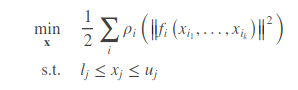
其在工程和科学领域有非常广泛的应用，比如统计学中的曲线拟合，或者在计算机视觉中依据图像进行三维模型的构建等

使用流程

使用Ceres求解非线性优化问题，可以分为三个步骤：

1. 构建代价函数（cost function）
代价函数，也就是寻优的目标式。这个部分需要使用仿函数（functor）这一技巧来实现，做法是定义一个cost function的结构体，在结构体内重载（）运算符。关于仿函数的内容可以参考这篇博客：c++仿函数 functor

2.通过代价函数构建待求解的优化问题

3.配置求解器参数并求解问题
这个步骤就是设置方程怎么求解、求解过程是否输出等

二、举例

2.1、使用ceres求取函数的最小值（为方便教学，函数选取的非常简单）

很容易算出这个最小值在x等于10处，但是简单的问题更适合用来说来用法

先看源码：

#include <iostream>
#include <ceres/ceres.h>

using namespace std;
using namespace ceres;

//第一部分：构建代价函数 -- 这个是我们自己构造，可能还有很多残差，都可以按类写一个代价函数
struct CostFunctor {
    template <typename T>
   //operators是一种模板方法，其假定所的输入输出都变为T的格式
  //其中x为带估算的参数，residual是残差
    bool operator()(const T* const x, T* residual) const {
        residual[0] = T(10.0) - x[0]; //这里的T[10.0]，可以将10 转换位所需的T格式，如double，Jet等
        return true;
    }
};




//主函数
int main(int argc, char** argv) {
    google::InitGoogleLogging(argv[0]);

    // 寻优参数x的初始值，为5
    double initial_x = 5.0;
    double x = initial_x;


    // 第二部分：构建寻优问题
    // 设置好的残差计算的公式，使用auto-differentiation选项去获得导数（雅克比）.
    Problem problem;
    CostFunction* cost_function =
     //注意：costFunctor是前面定义的f(x)=10-x。
     //使用自动求导，将之前的代价函数结构体传入，第一个1是待测参量的维数，第二个1是每个待测参量的size
     // 比如有两个参量。第一个为m，大小9；第二个c，大小为3。那么就是<CostFunctor, 2, 9，3>
            new AutoDiffCostFunction<CostFunctor, 1, 1>(new CostFunctor); 
    problem.AddResidualBlock(cost_function, NULL, &x); //向问题中添加误差项，本问题比较简单，添加一个就行。


    //第三部分： 配置并运行求解器
    Solver::Options options;
    options.linear_solver_type = ceres::DENSE_QR; //使用得是稠密的QR分解方式
    options.minimizer_progress_to_stdout = true;//输出到cout
    Solver::Summary summary;//优化信息
    Solve(options, &problem, &summary);//求解!!!

    std::cout << summary.BriefReport() << "\n";//输出优化的简要信息
    //最终结果
    std::cout << "x : " << initial_x
              << " -> " << x << "\n";
    return 0;
}

本部分的官方参照代码在examples/helloworld.cc
笔者在ubuntumate 18.04下进行验证，结果为：

iter      cost      cost_change  |gradient|   |step|    tr_ratio  tr_radius  ls_iter  iter_time  total_time
   0  4.512500e+01    0.00e+00    9.50e+00   0.00e+00   0.00e+00  1.00e+04       0    5.33e-04    3.46e-03
   1  4.511598e-07    4.51e+01    9.50e-04   9.50e+00   1.00e+00  3.00e+04       1    5.00e-04    4.05e-03
   2  5.012552e-16    4.51e-07    3.17e-08   9.50e-04   1.00e+00  9.00e+04       1    1.60e-05    4.09e-03
Ceres Solver Report: Iterations: 2, Initial cost: 4.512500e+01, Final cost: 5.012552e-16, Termination: CONVERGENCE
x : 0.5 -> 10

2.2、ceres在powell法上的实现

接下来介绍一个较为复杂的问题，鲍威尔优化算法。有兴趣的可以查询其算法细节，本文主要是针对ceres的使用。
参数为 x = [x1, x2, x3, x4], 具体的函数为：

1. 构建代价函数（cost function）

struct F1 {
  template <typename T> bool operator()(const T* const x1,
                                        const T* const x2,
                                        T* residual) const {
    // f1 = x1 + 10 * x2;
    residual[0] = x1[0] + 10.0 * x2[0];
    return true;
  }
};

struct F2 {
  template <typename T> bool operator()(const T* const x3,
                                        const T* const x4,
                                        T* residual) const {
    // f2 = sqrt(5) (x3 - x4)
    residual[0] = sqrt(5.0) * (x3[0] - x4[0]);
    return true;
  }
};

struct F3 {
  template <typename T> bool operator()(const T* const x2,
                                        const T* const x3,
                                        T* residual) const {
    // f3 = (x2 - 2 x3)^2
    residual[0] = (x2[0] - 2.0 * x3[0]) * (x2[0] - 2.0 * x3[0]);
    return true;
  }
};

struct F4 {
  template <typename T> bool operator()(const T* const x1,
                                        const T* const x4,
                                        T* residual) const {
    // f4 = sqrt(10) (x1 - x4)^2
    residual[0] = sqrt(10.0) * (x1[0] - x4[0]) * (x1[0] - x4[0]);
    return true;
  }
};

2.通过代价函数构建待求解的优化问题

 Problem problem;
  // 还是用autoDiff的方式来求解导数，前面是costfunction的规模，后面是相关的参量，使用&来表明
  problem.AddResidualBlock(new AutoDiffCostFunction<F1, 1, 1, 1>(new F1),NULL,&x1, &x2);
  problem.AddResidualBlock(new AutoDiffCostFunction<F2, 1, 1, 1>(new F2),NULL,&x3, &x4);
  problem.AddResidualBlock(new AutoDiffCostFunction<F3, 1, 1, 1>(new F3), NULL,&x2, &x3);
  problem.AddResidualBlock(new AutoDiffCostFunction<F4, 1, 1, 1>(new F4),NULL,&x1, &x4);

3.配置求解器参数并求解问题

//Solver的配置类
Solver::Options options;
  LOG_IF(FATAL, !ceres::StringToMinimizerType(FLAGS_minimizer,
                                              &options.minimizer_type))
      << "Invalid minimizer: " << FLAGS_minimizer
      << ", valid options are: trust_region and line_search.";

  options.max_num_iterations = 100;//设置最大迭代次数
  options.linear_solver_type = ceres::DENSE_QR;//使用稠密QR方法解决
  options.minimizer_progress_to_stdout = true;//可以输出过程变量

  std::cout << "Initial x1 = " << x1
            << ", x2 = " << x2
            << ", x3 = " << x3
            << ", x4 = " << x4
            << "\n";

  // 运行solver!
  Solver::Summary summary;//用来放中间报告
  Solve(options, &problem, &summary);

  std::cout << summary.FullReport() << "\n";
  std::cout << "Final x1 = " << x1
            << ", x2 = " << x2
            << ", x3 = " << x3
            << ", x4 = " << x4
            << "\n";

运行结果为：

Final x1 = 0.000292189, x2 = -2.92189e-05, x3 = 4.79511e-05, x4 = 4.79511e-05

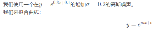
2.3、ceres在曲线拟合（Curve Fitting）中的实现

本部分为本笔记的重点，是我们第一次真正意义上的使用ceres解决非线性最小二乘问题，当然，结构是还是一致的，只需要稍加改动就可以实现。
数据来源：

1. 构建代价函数（cost function）

和前文一致，先建立损失函数，此处和前面不同的是第一次引入了数据，所以residual和前面有所区别，但这个位真正的非线性最小二乘的结构。

struct ExponentialResidual {
//定义数据的x和y的析构函数
  ExponentialResidual(double x, double y)
      : x_(x), y_(y) {}

  template <typename T>
  //两个待估参量m，c类型为指向T* 的指针
  bool operator()(const T* const m, const T* const c, T* residual) const {
   	//残差为一组数据中 r = y - f(x)
    residual[0] = T(y_) - exp(m[0] * T(x_) + c[0]);
    return true;
  }

 private:
  // 一组观测样本
  const double x_;
  const double y_;
};

2.通过代价函数构建待求解的优化问题

//设置初值
double m = 0.0;
double c = 0.0;
//构建最小二乘问题
Problem problem;
for (int i = 0; i < kNumObservations; ++i) {
  CostFunction* cost_function =
  		//残差维度为1，m维度为1，c维度为1：这就是三个1的意思
       new AutoDiffCostFunction<ExponentialResidual, 1, 1, 1>(
       //data中偶数位存放x的样本值，奇数位存放y的样本值
           new ExponentialResidual(data[2 * i], data[2 * i + 1]));
           //残差的参量是m和c
  problem.AddResidualBlock(cost_function, NULL, &m, &c);
}

3.配置求解器参数并求解问题

  Solver::Options options;
  options.max_num_iterations = 25;
  options.linear_solver_type = ceres::DENSE_QR;
  options.minimizer_progress_to_stdout = true;

  Solver::Summary summary;
  Solve(options, &problem, &summary);
  std::cout << summary.BriefReport() << "\n";
  std::cout << "Initial m: " << 0.0 << " c: " << 0.0 << "\n";
  std::cout << "Final   m: " << m << " c: " << c << "\n";

4、结果及分析

完整代码为：

#include "ceres/ceres.h"
#include "glog/logging.h"

using ceres::AutoDiffCostFunction;
using ceres::CostFunction;
using ceres::Problem;
using ceres::Solver;
using ceres::Solve;

// Data generated using the following octave code.
//   randn('seed', 23497);
//   m = 0.3;
//   c = 0.1;
//   x=[0:0.075:5];
//   y = exp(m * x + c);
//   noise = randn(size(x)) * 0.2;
//   y_observed = y + noise;
//   data = [x', y_observed'];

const int kNumObservations = 67;
const double data[] = {
  0.000000e+00, 1.133898e+00,
  7.500000e-02, 1.334902e+00,
  1.500000e-01, 1.213546e+00,
  2.250000e-01, 1.252016e+00,
  3.000000e-01, 1.392265e+00,
  3.750000e-01, 1.314458e+00,
  4.500000e-01, 1.472541e+00,
  5.250000e-01, 1.536218e+00,
  6.000000e-01, 1.355679e+00,
  6.750000e-01, 1.463566e+00,
  7.500000e-01, 1.490201e+00,
  8.250000e-01, 1.658699e+00,
  9.000000e-01, 1.067574e+00,
  9.750000e-01, 1.464629e+00,
  1.050000e+00, 1.402653e+00,
  1.125000e+00, 1.713141e+00,
  1.200000e+00, 1.527021e+00,
  1.275000e+00, 1.702632e+00,
  1.350000e+00, 1.423899e+00,
  1.425000e+00, 1.543078e+00,
  1.500000e+00, 1.664015e+00,
  1.575000e+00, 1.732484e+00,
  1.650000e+00, 1.543296e+00,
  1.725000e+00, 1.959523e+00,
  1.800000e+00, 1.685132e+00,
  1.875000e+00, 1.951791e+00,
  1.950000e+00, 2.095346e+00,
  2.025000e+00, 2.361460e+00,
  2.100000e+00, 2.169119e+00,
  2.175000e+00, 2.061745e+00,
  2.250000e+00, 2.178641e+00,
  2.325000e+00, 2.104346e+00,
  2.400000e+00, 2.584470e+00,
  2.475000e+00, 1.914158e+00,
  2.550000e+00, 2.368375e+00,
  2.625000e+00, 2.686125e+00,
  2.700000e+00, 2.712395e+00,
  2.775000e+00, 2.499511e+00,
  2.850000e+00, 2.558897e+00,
  2.925000e+00, 2.309154e+00,
  3.000000e+00, 2.869503e+00,
  3.075000e+00, 3.116645e+00,
  3.150000e+00, 3.094907e+00,
  3.225000e+00, 2.471759e+00,
  3.300000e+00, 3.017131e+00,
  3.375000e+00, 3.232381e+00,
  3.450000e+00, 2.944596e+00,
  3.525000e+00, 3.385343e+00,
  3.600000e+00, 3.199826e+00,
  3.675000e+00, 3.423039e+00,
  3.750000e+00, 3.621552e+00,
  3.825000e+00, 3.559255e+00,
  3.900000e+00, 3.530713e+00,
  3.975000e+00, 3.561766e+00,
  4.050000e+00, 3.544574e+00,
  4.125000e+00, 3.867945e+00,
  4.200000e+00, 4.049776e+00,
  4.275000e+00, 3.885601e+00,
  4.350000e+00, 4.110505e+00,
  4.425000e+00, 4.345320e+00,
  4.500000e+00, 4.161241e+00,
  4.575000e+00, 4.363407e+00,
  4.650000e+00, 4.161576e+00,
  4.725000e+00, 4.619728e+00,
  4.800000e+00, 4.737410e+00,
  4.875000e+00, 4.727863e+00,
  4.950000e+00, 4.669206e+00,
};

struct ExponentialResidual {
  ExponentialResidual(double x, double y)
      : x_(x), y_(y) {}

  template <typename T> bool operator()(const T* const m,
                                        const T* const c,
                                        T* residual) const {
    residual[0] = y_ - exp(m[0] * x_ + c[0]);
    return true;
  }

 private:
  const double x_;
  const double y_;
};

int main(int argc, char** argv) {
  google::InitGoogleLogging(argv[0]);

  double m = 0.0;
  double c = 0.0;

  Problem problem;
  for (int i = 0; i < kNumObservations; ++i) {
    problem.AddResidualBlock(
        new AutoDiffCostFunction<ExponentialResidual, 1, 1, 1>(
            new ExponentialResidual(data[2 * i], data[2 * i + 1])),
        NULL,
        &m, &c);
  }

  Solver::Options options;
  options.max_num_iterations = 25;
  options.linear_solver_type = ceres::DENSE_QR;
  options.minimizer_progress_to_stdout = true;

  Solver::Summary summary;
  Solve(options, &problem, &summary);
  std::cout << summary.BriefReport() << "\n";
  std::cout << "Initial m: " << 0.0 << " c: " << 0.0 << "\n";
  std::cout << "Final   m: " << m << " c: " << c << "\n";
  return 0;

输出结果为：

Final   m: 0.291861 c: 0.131439

可以看出，结果与真实的曲线m = 0.3 m=0.3m=0.3 c = 0.1 c= 0.1c=0.1有一定的差别，这正好说明了拟合的正确性，因为我们添加了高斯噪音。
可视化的结果为：

在这里插入图片描述

2.4、ceres在 BA 的实现

https://blog.csdn.net/hltt3838/article/details/109642247

他人是一面镜子，保持谦虚的态度

关注

1
点赞
踩
17

收藏

觉得还不错? 一键收藏
0
评论
Ceres Solver 具体案例分析

参考：https://blog.csdn.net/u014709760/article/details/88091720/一、简介本篇博客结合例子详细介绍一下 Ceres库的基本使用方法Ceres 可以解决边界约束鲁棒非线性最小二乘法优化问题，其概念可表达如下：其在工程和科学领域有非常广泛的应用，比如统计学中的曲线拟合，或者在计算机视觉中依据图像进行三维模型的构建等其中：别忘了。。。。。使用流程使用Ceres求解非线性优化问题，可以分为三个...
复制链接

扫一扫