


文章目录
DCN 可变形卷积
deformable attention 灵感来源可变形卷积,先来看看什么是可变形卷积DCN?
DCN 论文地址
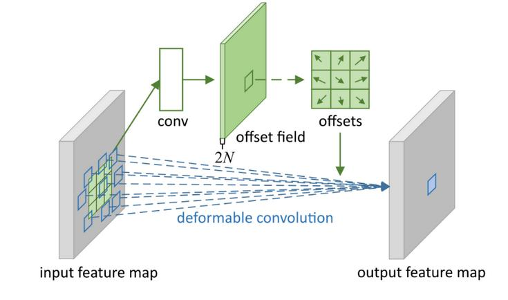
大概就像图中所示,传统的CNN 卷积核是固定的,假设为N = 3 x3,所以邻域9个采样点位置就是固定的。可变形卷积目的就是动态生成这9个采样位置。
首先特征图经过卷积层,这个和传统CNN没区别,然后生成与特征图一样大小的位置偏移网络,channel = N * 2,表示在原有9个固定采样点上的x, y 偏移。
得到偏移量后再回到原始特征图上进行插值采样,进行采样点卷积,得到当前特征点的输出值。
思考:为什么通过特征图能学到位置偏移?
对于深度学习来说,学习的目标值与输入的特征一定是强相关的,例如我们学习A特征点处的位置偏移,本质上就是学习与A特征点强相关的(attention)特征点(例如我们学习物体到边界偏移,边界特征为B)所在的位置。理论上是需要A,B两个特征作为先验,才能学习到他们的位置偏移,但是我们的输入只有当前A特征,B特征是通过先有位置索引才能找到,也就是说只给定A特征,如果你没有预期你想要的B特征长什么样(所谓的学习目标不明确),那这个位置偏移量也是无法学习出来的, 是不是很像先有鸡还是先有蛋的问题?从特征A出发,到底是先有边界特征B才有位置偏移还是先有位置偏移才有边界特征B。不知道大家有没有做过这方面的思考和疑惑?
这个问题我思考了许久,理解不了也无法理解后面的deformable attention 中的生成offset。
我认为的是,首先特征图不是原始图像,它是已经经过一定层CNN卷积后生成的特征,所以在局部区域,特征之间的信息是强相关的。也就是上述问题中特征点A(中心)与特征点B(边界)是强相关的。因为经过多成卷积,其实局部特征之间已经有一定的attention。也就是说,只给定特征A,它是能感受到它所在的边界在哪里,而不需要边界特征B作为输入,因为A特征所在位置经过多次卷积后其实已经融合了边界B特征的信息。如果 A , B 完全独立,那么我认为这个偏移量是无法学习出来的。
最后在边界约束(loss)的监督下,从A位置出发总优先取位于边界的特征B进行融合,而不是固定卷积窗口超出边界的特征,所以在卷积信息融合上(卷积本质就是信息融合后提纯),可变形卷积就体现出融合信息更加相关的优势。
单尺度 deformable attention
对于 Transformer attention 来说,最重要的信息就是Query, Key, Value了。
在self-attention 中,Query 和 Key 都是通过输入向量tokens进行生成,并进行全局上的attention 产生 attention 权重,得到每个token 相对其他token的注意力权重。 事先我们并不知道哪个token 对当前token 的贡献权重有多大,所以两两token 之间都交叉计算一遍,得到对应的权重W。
deformable attention 是局部自注意力,理论上attention 是通过局部选择的 token (这里的token为特征图上一个点)去产生 局部的Query , Key, Value, 得到局部的attention权重W后作用在局部的Value上。但是局部的token位置是未知的,需要模型去学习他的位置。最后我们要的是attention权重W,以及attention token 的 Value。既然attention权重W是先学习出Query , Key后产生, 而对应的Query , Key,也是先通过学习位置得到对应的token 后产生,那不如一步到位直接从特征图token中学习出attention权重W吧。
所以deformable attention 不直接产生 Query , Key, 而是直接学习以下两个:
1、相对reference point 的位置偏移, 这个主要是获取 attention token 。
2、对应每一个位置偏移得到的Value的权重W。
事实上在学习位置offset和对应的权重W时,我们事先也并不知道哪个token与当前token (reference point)是强相关的,那么它的位置偏移怎么能够精准学到呢?这就是我在前面DCN那里提到的问题。
理论讲差不多了,具体看细节。
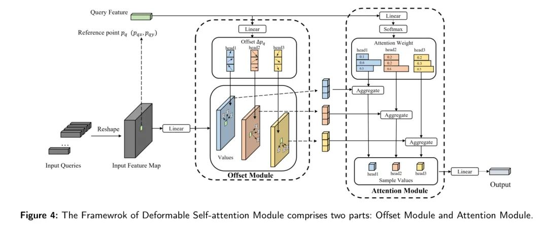
首先将CNN 后的特征图进行Linear 展开,每个特征点作为一个token。

1、每个特征点分成8个方向,每个方向上提取4个attention 特征点,那么总计就是要学习 N = 8 *4 = 32 个点的位置偏移。
2、对应的,每个特征点位置也要学习对应的 32 个权重值。
3、得到的位置偏移offset + referenpoint(还要经过插值,因为学出来是浮点的) 就可以索引到对应的attention token上。注意这里的位置偏移offset 是相对原图的归一化值,这个好处就是不同尺度特征图下同一位置的偏移offsets是相同的,也能更加方便网络学习。
4、把对应的attention W 乘以 attention token 的 Value,concat各个head(方向)上的结果, 就得到当前token 的 attention 输出。
多尺度(multiscale) deformable attention
多尺度是用于小目标检测的常规手段。加入多尺度后的deformable attention 能将多个尺度的信息直接融合,也不需要类似FPN 等neck 结构。
与单尺度不同的是,multiscale deformable attention 需要在不同的尺度上进行 deformable attention 。
1、生成多尺度特征:

使用 backbone + 二维函数式位置编码(也可换成可学习的)+ 尺度层级位置编码(可学习的产出不同尺度的特征图。
2、所有特征图上的像素点展开成一排token向量,作为输入。假设共4个scale level, 输入token个数为 :Len_q = L1 + L2 + L3 + L4
3、和单尺度一样,每个token 都要学习位置偏移和对应attention weight。不同的是当前尺度的 token 也会学习它在其他尺度下的位置偏移和权重。
学习位置偏移输出通道为:
C_offset = n_levels * n_points * n_head * 2
sampling_offsets = self.sampling_offsets(query).view(N, Len_q, self.n_heads, self.n_levels, self.n_points, 2)
学习attention weight 输出通道为:
C_w = n_levels * n_points * n_head
 attention_weights = self.attention_weights(query).view(N, Len_q, self.n_heads, self.n_levels * self.n_points)
 attention_weights = F.softmax(attention_weights, -1).view(N, Len_q, self.n_heads, self.n_levels, self.n_points)
最后对所有尺度上的attention weight 做softmax,因为当前尺度也会融合其他尺度的特征信息,融合力度由attention weight 决定,所以形成了多尺度信息融合而不需要FPN neck。
4、插值得到偏移量,取出对应位置的Value
对某个token , 生成 n_levels * n_points * n_head 个 位置偏移,每个尺度上有n_points * n_head 个位置偏移,因为这些偏移量来自不同的特征图,所以对应尺度的位置偏移要回到对应的尺度上,并在对应的尺度上取出Value。
#输入参考点坐标:param reference_points:(N, Length_{query}, n_levels, 2)
if reference_points.shape[-1] == 2:
            offset_normalizer = torch.stack([input_spatial_shapes[..., 1], input_spatial_shapes[..., 0]], -1)
            sampling_locations = reference_points[:, :, None, :, None, :] \
                                 + sampling_offsets / offset_normalizer[None, None, None, :, None, :]
elif reference_points.shape[-1] == 4:
     sampling_locations = reference_points[:, :, None, :, None, :2] \
                          + sampling_offsets / self.n_points * reference_points[:, :, None, :, None, 2:] * 0.5
这样 Len_q 个token,每个token就得到 n_levels * n_points * n_head 个Value 。
5、在每个head(方向)上,attention_weights *value, 此时会融合多个尺度的Value,得到当前head 的输出。然后把各个head 的结果 concat (shape = (Len_q, n_head, hidden_dim), hidden_dim 为 Value 的通道数)最后reshape 成 (Len_q,n_head * hidden_dim), 得到当前token 的 deformable attention后最终的输出。
注意:实际代码中Value 的输入通道为n_head * hidden_dim, 计算过程会将value向量按head拆开,相当一个Value变成不同方向的Value,然后才与attention_weights进行计算,计算完后按head(方向)concat起来,最后输出通道仍是n_head * hidden_dim。
# =============================================================================
# 将value向量按head拆开
# value:尺寸为:(B, sum(所有特征图的token数量), nheads, d_model//n_heads)
# =============================================================================
value = value.view(N, Len_in, self.n_heads, self.d_model // self.n_heads)
# =====
 # (4)最后把output处理成:(B, nheads*head_dim, sum(tokens))
 # ================================================================================
 output = (torch.stack(sampling_value_list, dim=-2).flatten(-2) * attention_weights).sum(-1).view(N_, M_*D_, Lq_)
 # ================================================================================
 # 经过转置以后,最后的deformable attention的output变成(B, sum(tokens),nheads*head_dim)
 # ================================================================================
 return output.transpose(1, 2).contiguous()
整个deformable attention 的pipline 如下:
分别是采样位置(Sample Location)、注意力权重(Attention Weights)、映射后的 Value 特征、多尺度特征每层特征起始索引位置、多尺度特征图的空间大小(便于将采样位置由归一化的值变成绝对位置);
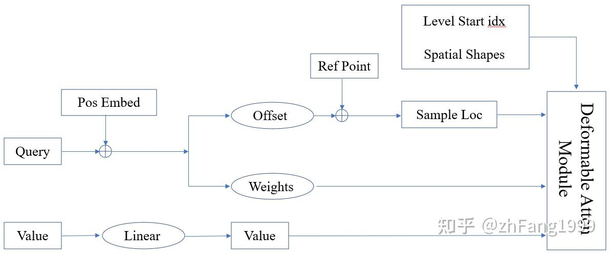 采样点的位置相对于参考点的偏移量和每个采样点在加权时的比重均是靠 Query 经过 Linear 层学习得到的。
当前deformable attention已经封装成CUDA模块,只要将输入对齐,就可以直接调用。
精华代码
:deformbale attention
class MSDeformAttn(nn.Module):
    def __init__(self, d_model=256, n_levels=4, n_heads=8, n_points=4):
        """
        Multi-Scale Deformable Attention Module
        :param d_model      hidden dimension
        :param n_levels     number of feature levels (特征图的数量)
        :param n_heads      number of attention heads
        :param n_points     number of sampling points per attention head per feature level
                            每个特征图的每个attention上需要sample的points数量
        """
        super().__init__()
        if d_model % n_heads != 0:
            raise ValueError('d_model must be divisible by n_heads, but got {} and {}'.format(d_model, n_heads))
        _d_per_head = d_model // n_heads
        # you'd better set _d_per_head to a power of 2 which is more efficient in our CUDA implementation
        if not _is_power_of_2(_d_per_head):
            warnings.warn("You'd better set d_model in MSDeformAttn to make the dimension of each attention head a power of 2 "
                          "which is more efficient in our CUDA implementation.")

        self.im2col_step = 64

        self.d_model = d_model
        self.n_levels = n_levels
        self.n_heads = n_heads
        self.n_points = n_points

        # =============================================================================
        # 每个query在每个head每个特征图(n_levels)上都需要采样n_points个偏移点,每个点的像素坐标用(x,y)表示
        # =============================================================================
        self.sampling_offsets = nn.Linear(d_model, n_heads * n_levels * n_points * 2)

        # =============================================================================
        # 每个query用于计算注意力权重的参数矩阵
        # =============================================================================
        self.attention_weights = nn.Linear(d_model, n_heads * n_levels * n_points)

        # =============================================================================
        # value的线性变化
        # =============================================================================
        self.value_proj = nn.Linear(d_model, d_model)

        # =============================================================================
        # 输出结果的线性变化
        # =============================================================================
        self.output_proj = nn.Linear(d_model, d_model)

        self._reset_parameters()

    def _reset_parameters(self):
        # =============================================================================
        # sampling_offsets的权重初始化为0
        # =============================================================================
        constant_(self.sampling_offsets.weight.data, 0.)
        # =============================================================================
        # thetas: 尺寸为(nheads, ),假设nheads = 8,则值为:
        # tensor([0*(pi/4), 1*(pi/4), 2*(pi/4), ..., 7 * (pi/4)])
        # 好似把一个圆切成了n_heads份,用于表示一个图的nheads个方位
        # =============================================================================
        thetas = torch.arange(self.n_heads, dtype=torch.float32) * (2.0 * math.pi / self.n_heads)
        # =============================================================================
        # grid_init: 尺寸为(nheads, 2),即每一个方位角的cos和sin值,例如:
        # tensor([[ 1.0000e+00,  0.0000e+00],
        #         [ 7.0711e-01,  7.0711e-01],
        #         [-4.3711e-08,  1.0000e+00],
        #         [-7.0711e-01,  7.0711e-01],
        #         [-1.0000e+00, -8.7423e-08],
        #         [-7.0711e-01, -7.0711e-01],
        #         [ 1.1925e-08, -1.0000e+00],
        #         [ 7.0711e-01, -7.0711e-01]])
        # =============================================================================
        grid_init = torch.stack([thetas.cos(), thetas.sin()], -1)
        # =============================================================================
        # 第一步:
        # grid_init / grid_init.abs().max(-1, keepdim=True)[0]:计算8个head的坐标偏移,尺寸为torch.Size([n_heads, 2])
        # 结果为:
        # tensor([[ 1.,  0.],
        #         [ 1.,  1.],
        #         [0.,  1.],
        #         [-1.,  1.],
        #         [-1., 0.],
        #         [-1., -1.],
        #         [0., -1.],
        #         [1., -1]])
        # 然后把这个数据广播给每个n_level的每个n_point
        # 最后grid_init尺寸为:(nheads, n_levels, n_points, 2)
        # 这意味着:在第一个head上,每个level上,每个偏移点的偏移量都是(1,0)
        #         在第二个head上,每个level上,每个偏移点的偏移量都是(1,1),以此类推
        # =============================================================================
        grid_init = (grid_init / grid_init.abs().max(-1, keepdim=True)[0]).view(self.n_heads, 1, 1, 2).repeat(1, self.n_levels, self.n_points, 1)
        # =============================================================================
        # 每个参考点的初始化偏移量肯定不能一样,所以这里第i个参考点的偏移量设为:
        # (i,0), (i,i), (0,i)...(i,-i)
        # grid_init尺寸依然是:(nheads, n_levels, n_points, 2)
        # 现在意味着:在第一个head上,每个level上,第一个偏移点偏移量是(1,0), 第二个是(2,0),第三个是(3,0), 第四个是(4,0)
        #           在第二个head上,每个level上,都一个偏移点偏移量是(1,1), 第二个是(2,2), 第三个是(3,3), 第四个是(4,4)
        # =============================================================================
        for i in range(self.n_points):
            grid_init[:, :, i, :] *= i + 1
        # =============================================================================
        # 初始化sampling_offsets的bias,但其不参与训练。尺寸为(nheads * n_levels * n_points * 2,)
        # =============================================================================
        with torch.no_grad():
            self.sampling_offsets.bias = nn.Parameter(grid_init.view(-1))

        # =============================================================================
        # 其余参数的初始化
        # =============================================================================
        constant_(self.attention_weights.weight.data, 0.)
        constant_(self.attention_weights.bias.data, 0.)
        xavier_uniform_(self.value_proj.weight.data)
        constant_(self.value_proj.bias.data, 0.)
        xavier_uniform_(self.output_proj.weight.data)
        constant_(self.output_proj.bias.data, 0.)

    def forward(self, query, reference_points, input_flatten, input_spatial_shapes, input_level_start_index, input_padding_mask=None):
        """


        Args:
            query:原始输入数据 + 位置编码后的结果,尺寸为(B, sum(所有特征图的token数量), 256)
                   sum(所有特征图的token数量)其实就是sum(H_*W_)

            reference_poins:尺寸为(B, sum(所有特征图的token数量), level_num, 2)。表示对于                                batch中的每一条数据的每个token,它在不同特征层上的坐标表示。
                            请一定参见get_reference_points函数相关注释

            input_flatten: 原始输入数据,尺寸为(B, sum(所有特征图的token数量), 256)

            input_spatial_shapes: tensor,其尺寸为(level_num,2)。 表示原始特征图的大小。
                                  其中2表是Hi, Wi。例如:
                                  tensor([[94, 86],
                                          [47, 43],
                                          [24, 22],
                                          [12, 11]])

            input_level_start_index: 尺寸为(level_num, )
                                     表示每个level的起始token在整排token中的序号,例如:
                                     tensor([0,  8084, 10105, 10633])

            input_padding_mask:     mask信息,(B, sum(所有特征图的token数量))

        """
        # =============================================================================
        # N:batch_size
        # len_q: query数量,在encoder attention中等于len_in
        # len_in: 所有特征图组成的token数量
        # =============================================================================
        N, Len_q, _ = query.shape
        N, Len_in, _ = input_flatten.shape
        # 声明所有特征图的像素数量 = token数量
        assert (input_spatial_shapes[:, 0] * input_spatial_shapes[:, 1]).sum() == Len_in

        # =============================================================================
        # self.value_proj:线性层,可理解成是Wq, 尺寸为(d_model, d_model)
        # value:v值,尺寸为(B, sum(所有特征图的token数量), 256)
        # =============================================================================
        value = self.value_proj(input_flatten)
        # =============================================================================
        # 对于V值,将padding的部分用0填充(那个token向量变成0向量)
        # =============================================================================
        if input_padding_mask is not None:
            value = value.masked_fill(input_padding_mask[..., None], float(0))
        # =============================================================================
        # 将value向量按head拆开
        # value:尺寸为:(B, sum(所有特征图的token数量), nheads, d_model//n_heads)
        # =============================================================================
        value = value.view(N, Len_in, self.n_heads, self.d_model // self.n_heads)
        # =============================================================================
        # self.sampling_offsets:偏移点的权重,尺寸为(d_model, n_heads * n_levels * n_points * 2)
        #                        【对于一个token,求它在每个head的每个level的每个偏移point上
        #                        的坐标结果(x, y)】
        # 由于sampling_offsets.weight.data被初始化为0,但sampling_offsets.bias.data却被初始化
        # 为我们设定好的偏移量,所以第一次fwd时,这个sampling_offsets是我们设定好的初始化偏移量
        # self.sampling_offsets(query) = (B, sum(所有特征图的token数量), d_model) *
        #                                (d_model, n_heads * n_levels * n_points * 2)
        #                              = (B, sum(所有特征图的token数量), n_heads * n_levels * n_points * 2)
        # =============================================================================
        sampling_offsets = self.sampling_offsets(query).view(N, Len_q, self.n_heads, self.n_levels, self.n_points, 2)
        # =============================================================================
        # self.attention_weights: 线性层,尺寸为(d_model, n_heads * n_levels * n_points),
        #                         初始化时weight和bias都被设为0
        # 因此attention_weights第一次做fwd时全为0
        # =============================================================================
        attention_weights = self.attention_weights(query).view(N, Len_q, self.n_heads, self.n_levels * self.n_points)
        # =============================================================================
        # attention_weights: 表示每一个token在每一个head的每一个level上,和它的n_points个偏移向量
        #                    的attention score。
        #                    初始化时这些attention score都是相同的
        # =============================================================================
        attention_weights = F.softmax(attention_weights, -1).view(N, Len_q, self.n_heads, self.n_levels, self.n_points)
        # =============================================================================
        # reference_points:尺寸为(B, sum(所有token数量), level_num, 2)
        # N, Len_q, n_heads, n_levels, n_points, 2
        # =============================================================================
        if reference_points.shape[-1] == 2:
            # ======================================================================
            # offset_normalizer: 尺寸为(level_num, 2),表示每个特征图的原始大小,坐标表达为(W_, H_)
            # ======================================================================
            offset_normalizer = torch.stack([input_spatial_shapes[..., 1], input_spatial_shapes[..., 0]], -1)
            # ======================================================================
            # 先介绍下三个元素:
            # reference_points[:, :, None, :, None, :]:
            #  尺寸为 (B, sum(token数量), 1, n_levels, 1,2)

            # sampling_offsets:
            # 尺寸为(B, sum(token数量), n_heads, n_levels, n_points, 2)

            # offset_normalizer[None,None,None,:,None,:]:
            # 尺寸为(1, 1, 1,n_levels, 1,2)

            # 再介绍下怎么操作的:
            # (1)sampling_offsets / offset_normalizer[None, None, None, :, None, :]:
            # 前者表示预测出来的偏移量(单位是像素绝对值)通过相除,把它变成像素归一化以后的维度
            #  (2) 加上reference_points:表示把该token对应的这个参考点做偏移,
            # 得到其在各个level上的n_points个偏移结果,偏移结果同样是用归一化的像素坐标来表示
            # sampling_locations:尺寸为(B, sum(tokens数量), nhead, n_levels, n_points, 2)
            # ======================================================================
            sampling_locations = reference_points[:, :, None, :, None, :] \
                                 + sampling_offsets / offset_normalizer[None, None, None, :, None, :]
        elif reference_points.shape[-1] == 4:
            sampling_locations = reference_points[:, :, None, :, None, :2] \
                                 + sampling_offsets / self.n_points * reference_points[:, :, None, :, None, 2:] * 0.5
        else:
            raise ValueError(
                'Last dim of reference_points must be 2 or 4, but get {} instead.'.format(reference_points.shape[-1]))
        output = MSDeformAttnFunction.apply(
            value, input_spatial_shapes, input_level_start_index, sampling_locations, attention_weights, self.im2col_step)
        output = self.output_proj(output)
        return output
attention 计算:
def ms_deform_attn_core_pytorch(value, value_spatial_shapes, sampling_locations, attention_weights):
    """
    Args:
        value: 尺寸为:(B, sum(所有特征图的token数量), nheads, d_model//n_heads)。对原始token做线性变化
               后的value值

        input_spatial_shapes: tensor,其尺寸为(level_num,2)。 表示原始特征图的大小。
                              其中2表是Hi, Wi。例如:
                              tensor([[94, 86],
                                      [47, 43],
                                      [24, 22],
                                      [12, 11]])
        sampling_locations:尺寸为(B, sum(tokens数量), nhead, n_levels, n_points, 2)。
                            每个token在每个head、level上的n_points个偏移点坐标(坐标是归一化的像素值),
                            每个坐标是按(w,h)表达的,注意不是(h,1)

        attention_weights: 尺寸为(B, sum(tokens数量), nheads, n_levels, n_points)
                           每个token在每个head、level上对n_points个偏移点坐标的注意力权重
    """
    # for debug and test only,
    # need to use cuda version instead
    N_, S_, M_, D_ = value.shape
    _, Lq_, M_, L_, P_, _ = sampling_locations.shape
    # ================================================================================
    # 截取出每个特征图的value
    # value_list: tuple[Tensor],value_list长度 = n_levels
    #             每个tensor尺寸为(B, sum(某个特征图token数量), nheads, d_model//n_heads)
    # ================================================================================
    value_list = value.split([H_ * W_ for H_, W_ in value_spatial_shapes], dim=1)
    # ================================================================================
    # 原来我们归一化后,坐标是在H=(0,1), W=(0,1)这个假设下的,现在我们想让H = (-1, 1), W = (-1,1),
    # 所以对所有的坐标也要做相应处理
    # sampling_grids: 尺寸依然是(B, sum(tokens数量), nhead, n_levels, n_points, 2)
    # ================================================================================
    sampling_grids = 2 * sampling_locations - 1
    sampling_value_list = []
    for lid_, (H_, W_) in enumerate(value_spatial_shapes):
        # (B, H_*W_, nheads, head_dim) -> (B, H_*W_, nheads*head_dim) -> (B, n_heads*head_dim, H_*W_) -> (B*nhead, head_dim, H_, W_)
        value_l_ = value_list[lid_].flatten(2).transpose(1, 2).reshape(N_*M_, D_, H_, W_)
        # (B, sum(所有token), nheads, n_poins, 2) -> (B, nheads, sum(所有token), n_points, 2) -> (B*nhead, sum(所有token), n_points, 2)
        sampling_grid_l_ = sampling_grids[:, :, :, lid_].transpose(1, 2).flatten(0, 1)
        #(B*nhead, head_dim, sum(所有token), n_points)
        sampling_value_l_ = F.grid_sample(value_l_, sampling_grid_l_,
                                          mode='bilinear', padding_mode='zeros', align_corners=False)
        sampling_value_list.append(sampling_value_l_)cc
    # (B, sum(token数量), nheads, n_levels, n_points) -> (B*nheads, sum(token数量), n_levels, n_points) -> (B, nheads, 1, sum(token数量), n_levels * n_points)
    attention_weights = attention_weights.transpose(1, 2).reshape(N_*M_, 1, Lq_, L_*P_)
    # ================================================================================
    # (1)torch.stack(sampling_value_list, dim=-2).flatten(-2):
    #  尺寸为(B*n_heads, head_dim, sum(token数量), n_levels*n_points)
    # (2)乘上attention_weights =
    #      (B*n_heads, head_dim, sum(token数量), n_levels*n_points) *
    #      (B*n_heads, 1, sum(token数量), n_levels*n_points)
    #       = (B*n_heads, head_dim, sum(token数量), n_levels*n_points)
    # (3).sum(-1): 处理后尺寸为(B*n_heads, head_dim, sum(token数量))
    # (4)最后把output处理成:(B, nheads*head_dim, sum(tokens))
    # ================================================================================
    output = (torch.stack(sampling_value_list, dim=-2).flatten(-2) * attention_weights).sum(-1).view(N_, M_*D_, Lq_)
    # ================================================================================
    # 经过转置以后,最后的deformable attention的output变成(B, sum(tokens),nheads*head_dim)
    # ================================================================================
    return output.transpose(1, 2).contiguous()
获取不同尺度参考点:
@staticmethod
    def get_reference_points(spatial_shapes, valid_ratios, device):
        """
        Args:
            spatial_shapes: tensor,其尺寸为(level_num,2)。 表示原始特征图的大小。
                            其中2表是Hi, Wi。例如:
                            tensor([[94, 86],
                                   [47, 43],
                                   [24, 22],
                                   [12, 11]])

            valid_ratios:      尺寸为(B, level_num, 2),
                               用于表示batch中的每条数据在每个特征图上,分别沿着H和W方向的
                               有效比例(有效 = 非padding部分)
                               例如特征图如下:
                               1, 1, 1, 0
                               1, 1, 1, 0
                               0, 0, 0, 0
                               则该特征图在H方向上的有效比例 = 2/3 = 0.6
                               在W方向上的有效比例 = 3/4 = 0.75

        """
        reference_points_list = []
        for lvl, (H_, W_) in enumerate(spatial_shapes):
            # =========================================================================
            # (1)torch.linspace(0.5, H_ - 0.5, H_): 可以看成按0.5像素单位把H方向切割成若干份
            # (2)torch.linspace(0.5, W_ - 0.5, W_): 可以看成按0.5像素单位把W方向切割成若干份
            #  例如设H_, W_ = 12, 16, 则(1)和(2)分别为:
            #  tensor([ 0.5000,  1.5000,  2.5000,  3.5000,  4.5000,  5.5000,  6.5000,               #           7.5000,  8.5000,  9.5000, 10.5000, 11.5000])
            #  tensor([ 0.5000,  1.5000,  2.5000,  3.5000,  4.5000,  5.5000,  6.5000,               #           7.5000,  8.5000,  9.5000, 10.5000, 11.5000, 12.5000, 13.5000,               #           14.5000, 15.5000])
            #
            # 你可以想成把一张特征图横向划几条线,纵向画几条线。对于一个像素格子,我们用其质心坐标
            # 表示它,这相当于是这些线的交界点
            #
            # 这里ref_y表示每个ref点的x坐标(H方向坐标),ref_x表示每个ref点的y坐标(W方向坐标)
            # (3) ref_y: 尺寸为(H_, W_), 形式如:
            # tensor([[ 0.5000,  0.5000,  0.5000,  0.5000,  0.5000,  0.5000,  0.5000,               #           0.5000, 0.5000,  0.5000,  0.5000,  0.5000,  0.5000,  0.5000,                #           0.5000,  0.5000],
            #         [ 1.5000,  1.5000,  1.5000,  1.5000,  1.5000,  1.5000,  1.5000,               #           1.5000,  1.5000,  1.5000,  1.5000,  1.5000,  1.5000,  1.5000,               ¥           1.5000,  1.5000],
            #         ...
            #         [11.5000, 11.5000, 11.5000, 11.5000, 11.5000, 11.5000, 11.5000,               #          11.5000,
            #          11.5000, 11.5000, 11.5000, 11.5000, 11.5000, 11.5000, 11.5000,               #          11.5000]])
            #
            # (4) ref_x:尺寸为(H_, W_),形式如:
            # tensor([[  0.5000,  1.5000,  2.5000,  3.5000,  4.5000,  5.5000,  6.5000,              #            7.5000,  8.5000,  9.5000, 10.5000, 11.5000, 12.5000, 13.5000,              #            14.5000, 15.5000],
            #         [  0.5000,  1.5000,  2.5000,  3.5000,  4.5000,  5.5000,  6.5000,              #            7.5000, 8.5000,  9.5000, 10.5000, 11.5000, 12.5000, 13.5000,               #            14.5000, 15.5000],
            #         ...(重复下去)
            # =========================================================================
            ref_y, ref_x = torch.meshgrid(torch.linspace(0.5, H_ - 0.5, H_, dtype=torch.float32, device=device),
                                          torch.linspace(0.5, W_ - 0.5, W_, dtype=torch.float32, device=device))

            # =========================================================================
            # 相当于每个像素格子都用其中心点的坐标来表示它
            #  ref_y.reshape(-1)[None]: 把(H_, W_)展平成(1, H_*W_)。
            #                           例如H_=12, W_=16, 则展平成(1, 192)
            # tensor([[ 0.5000,  0.5000,  0.5000,  0.5000,  0.5000,  0.5000,  0.5000,               #           0.5000,  0.5000,  0.5000,  0.5000,  0.5000,  0.5000,  0.5000,               #           0.5000,  0.5000,
            #           1.5000,  1.5000,  1.5000,  1.5000,  1.5000,  1.5000,  1.5000,               #           1.5000,  1.5000,  1.5000,  1.5000,  1.5000,  1.5000,  1.5000,               #           1.5000,  1.5000,
            #           ...
            #           11.5000, 11.5000, 11.5000, 11.5000, 11.5000, 11.5000, 11.5000,              #           11.5000, 11.5000, 11.5000, 11.5000, 11.5000, 11.5000, 11.5000,              #           11.5000, 11.5000]])
            #
            # ref_x.reshape(-1)[None]:把(H_, W_)展平成(1, H_*W_)。例子同上
            # tensor([[ 0.5000,  1.5000,  2.5000,  3.5000,  4.5000,  5.5000,  6.5000,               #           7.5000,  8.5000,  9.5000, 10.5000, 11.5000, 12.5000, 13.5000,               #           14.5000, 15.5000, 0.5000,  1.5000,  2.5000,  3.5000,  4.5000,               #           5.5000,  6.5000,  7.5000,  8.5000,  9.5000, 10.5000, 11.5000,               #           12.5000, 13.5000, 14.5000, 15.5000,
            #           ...
            #
            # valid_ratios[:, None, lvl, 1]:
            # 取出batch中所有数据在当前lvl这层特征图上,H方向的有效比例(有效=非padding)
            # 尺寸为(B, 1),例如:
            # tensor([[0.6667],
            # [0.6667],
            # [0.9167],
            # [1.0000]])
            # 乘上H_后表示实际有效的像素级长度
            # valid_ratios[:, None, lvl, 0]:也是同理
            #
            # ref_y: 尺寸为(B, H_ * W_)。
            #        表示对于batch中的每条数据,它在该lvl层特征图上一共有H_*W_个参考点,ref_y
            #        表示这些参考点最终在H方向上的像素坐标。【但这里像素坐标做了类似归一划的处理。
            #        ref_y = 原始H方向的绝对像素坐标/H方向上有效即非padding部分的绝对像素长度
            #        因此该值如果 > 1则说明该参考点在padding部分】
            # ref_x:尺寸为(B, H_ * W_)。同上
            # =========================================================================
            ref_y = ref_y.reshape(-1)[None] / (valid_ratios[:, None, lvl, 1] * H_)
            ref_x = ref_x.reshape(-1)[None] / (valid_ratios[:, None, lvl, 0] * W_)

            # =========================================================================
            # ref:尺寸为(B, H_*W_, 2),表示对于batch中的每条数据,它在该lvl层特征图上所有H_*W_个参考点的x,y坐标
            #     如上所说,该坐标已经处理成相对于有效像素长度的形式
            #    【特别注意!这里W和H换了位置!!!!!!】
            # =========================================================================
            ref = torch.stack((ref_x, ref_y), -1)
            reference_points_list.append(ref)
        # =========================================================================
        # 尺寸为:(B, sum(H_*W_), 2)。表示对于一个batch中的每一条数据,
        #       它在所有特征图上的参考点(数量为sum(H_*w))的像素坐标x,y。
        #       这里x,y都做过处理,表示该参考点相对于非padding部分的H,W的比值
        #       例如,如果x和y>1, 则说明该参考点在padding部分
        # =========================================================================
        reference_points = torch.cat(reference_points_list, 1)
        # =========================================================================
        # 尺寸为:(B, sum(H_*W_), level_num, 2)。表示对于batch中的每一条数据,
        #        它的每一个特征层上的归一化坐标,在其他特征层(也包括自己)上的所有归一化坐标
        # 假设对于某条数据:
        # 特征图1的高度为H1,有效高度为HE1,其上某个ref点x坐标为h1。则该ref点归一化坐标可以表示成h1/H1
        # 特征图2的高度为H2,有效高度为HE2,那么特征图1中的ref点在特征图2中,对应的归一化坐标应该是多少?
        # 【常规思路】:正常情况下,你可能觉得,我只要对每一张特征图上的像素点坐标都做归一化,然后对任意两张特征图,
        #             我取出像素点坐标一致的ref点,它不就能表示两张特征图的相同位置吗?
        # 【问题】:每张特征图padding的比例不一样,因此不能这么做。举例(参见草稿纸上的图)。特征图1上绝对像素
        #         位置3.5的点,在特征图2上的位置是2.1,在有效图部分之外
        # 【正确做法】:把特征图上的坐标表示成相对于有效部分的比例
        # 【解】:我们希望 h1/HE1 = h2/HE2,在此基础上我们再来求h2/H2
        #  则我们有:h2 = (h1/HE1) * HE2,进一步有
        #  (h2/H2) = (h1/HE1) * (HE2/H2),而(h1/HE1)就是reference_points[:, :, None],
        #                                  (HE2/H2)就是valid_ratios[:, None]
        # 所以,这里是先将不同特征图之间的映射转为“绝对坐标/有效长度”的表达,然后再转成该绝对坐标在整体长度上的比例
        # =========================================================================
        reference_points = reference_points[:, :, None] * valid_ratios[:, None]
        return reference_points


 830
830

 被折叠的 条评论
为什么被折叠?
被折叠的 条评论
为什么被折叠?
 到【灌水乐园】发言


