2、目标跟踪：卡尔曼滤波状态估计与更新

---

一、状态估计与更新

• 状态估计与更新：根据目标的先验模型和观测序列（摄像头、激光雷达、毫米波雷达等），对目标的状态进行估计与更新
  

二、卡尔曼滤波

2.1、简介

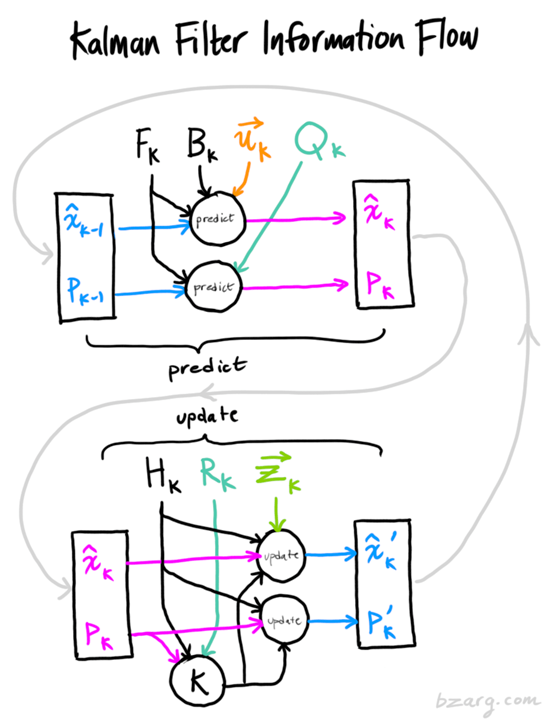
• 卡尔曼滤波本质上是一个数据融合算法（卡尔曼滤波的结果和传感器的探测结果），将具有同样测量目的、来自不同传感器或模型、具有不同单位的数据 融合 在一起（一般使用精度较高的测量值对模型预测的结果进行修正）得到一个更精确的估计值：

  • 首先，根据模型上一时刻的最优估计值来估计当前时刻的状态，得到模型在 当前时刻的先验估计值（prediction）
  • 然后，根据当前时刻的先验估计值和空间变换矩阵 H（状态到观测的变换矩阵 project），得到 观测空间的先验估计值
  • 最后，使用当前时刻传感器的测量值（measurement）来更正（update）这个估计值，得到 当前时刻的最优估计值

• 优点：占用内存小、速度快（除了前一个状态量外，不需要保留其它历史数据）

• 缺点：只能拟合线性高斯系统，对于非线性系统来说，可使用扩展卡尔曼滤波（多了一个把预测和测量部分进行线性化的过程）

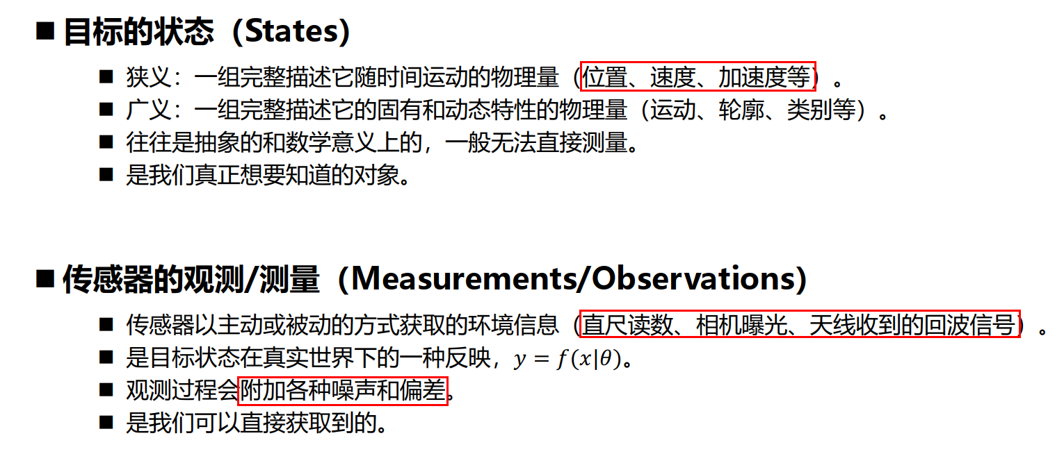
• 应用：比如跟踪目标，但目标的 位置、速度、加速度 的测量值往往在任何时候都有噪声。卡尔曼滤波利用目标的动态信息,设法去掉噪声的影响，得到一个关于目标位置的好的估计。这个估计可以是对当前目标位置的估计(滤波)，也可以是对将来位置的估计(预测)，也可以是对过去位置的估计(插值或平滑)

• Note：卡尔曼滤波是假设物体以某种单一的运动形式运动，不会存在突变的情况，所以现在 MOT 经常还是用在 行人和低速行驶的车辆等

---

2.2、prediction 部分（根据前一状态更新当前模型的状态及协方差矩阵）

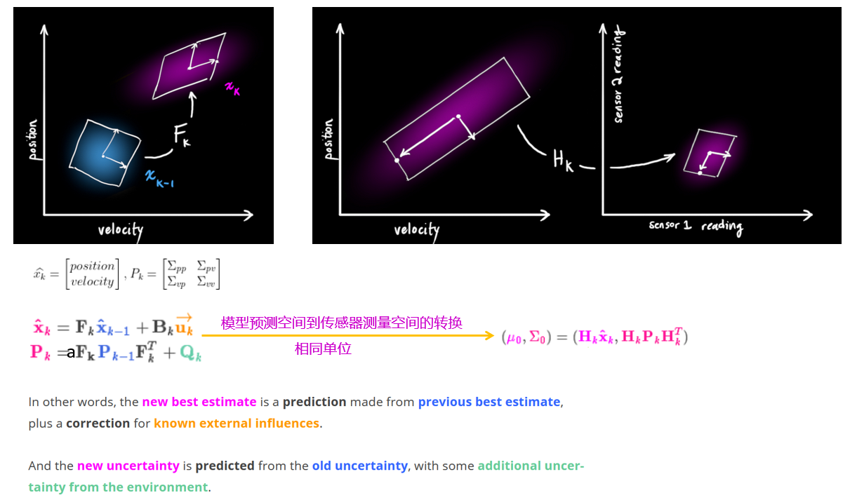
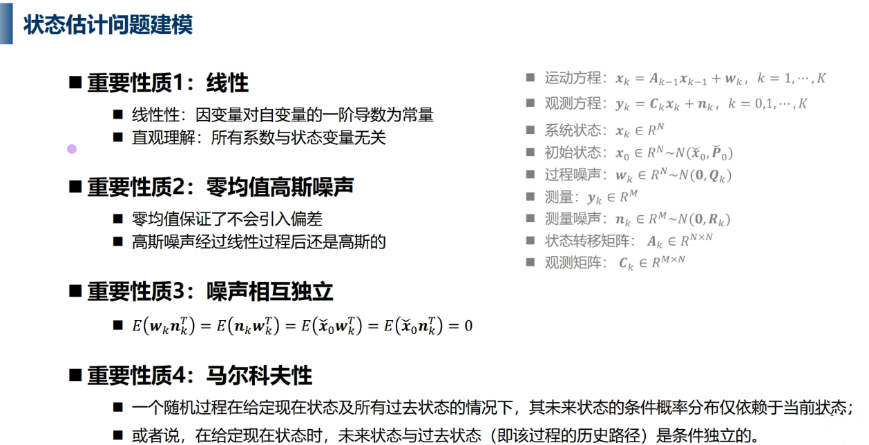
• 预测阶段：使用运动模型根据上一帧的状态变量来预测当前帧的状态变量（位置变，速度不变），与当前帧的检测结果计算代价矩阵后进行最优匹配。卡尔曼滤波假设两个变量（位置和速度）都是随机的，并且服从高斯分布，每个变量都有一个均值 $\mu$ 表示随机分布的中心（最可能的状态），以及方差 ${\sigma }^2$ 表示不确定性，相关变量的含义如下：
• x（8）：状态变量，表示某一时刻的状态（包含位置和速度）
• P（8, 8）：状态协方差矩阵，不仅包含了各个变量的不确定程度（方差），还描述了它们之间的相关性（正相关，两个变量趋向于同时增大或减小；负相关，一个变量增大时，另一个变量减小），根据观测值进行初始化，随 predict 不断变化
• F（8, 8）: 状态转移矩阵，将上一时刻的值转移到当前时刻
• Q（8, 8）：预测值噪声协方差矩阵，描述系统模型中的不确定性，反映了预测模型的运动估计误差，使用 mean h*权重初始化，随 predict mean 的变化不断变化
• B：控制输入矩阵（如果有外部控制输入），外部影响因素，线程模型中一般不用
• u：控制输入向量，外部影响因素，线程模型中一般不用
• a：遗忘系数，其作用在于调节对历史信息的依赖程度，越大对历史信息的依赖越小，线程模型中一般不用

---

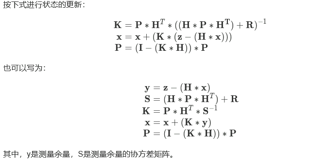
2.3、update（用传感器测量值来修正模型预测值）

使用当前帧的检测结果来修正预测的状态变量；更新后的状态变量为下一帧的预测做准备

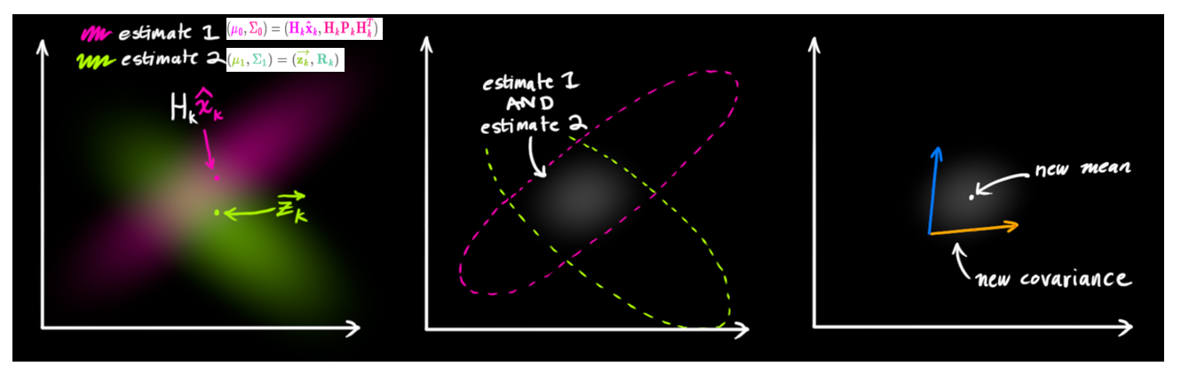
update 原理： 假设传感器的测量值和由前一状态得到的预测值都服从高斯分布，如果我们想知道这两种情况都可能发生的概率，将这两个高斯分布相乘就可以了（相当于取加权平均），相关变量的含义如下：

• H（4, 8）：状态到观测的变换矩阵（传感器读取的数据的单位和尺度有可能与我们要跟踪的状态的单位和尺度不一样，且观测变量比跟踪的少，比如没有速度变量；所以要用一个变换矩阵）
• z（4）：观测变量，表示传感器读到的数据
• R（4, 4）：传感器的 观测噪声协方差矩阵，描述测量过程中的噪声，反映了观测数据的不确定性；可以根据观测的置信度调整它 std = [(1 - confidence) * x for x in std]
• K（8, 4）：卡尔曼增益，它决定了系统在预测估计和测量估计之间如何加权，介于 0 和 1 之间；如果测量噪声 R 较大，卡尔曼增益会较小，意味着系统对新观测的信任较低，更多依赖于预测；如果测量噪声 R 较小，卡尔曼增益会较大，系统会更依赖新的测量值
  • 当 没有观测噪声（K=1） 时，相当于最优估计等于 观测值
  • 当 状态估计没有噪音（K=0） 时，相当于最优估计等于 预测值

• 融合高斯分布（公式推导）
  
  

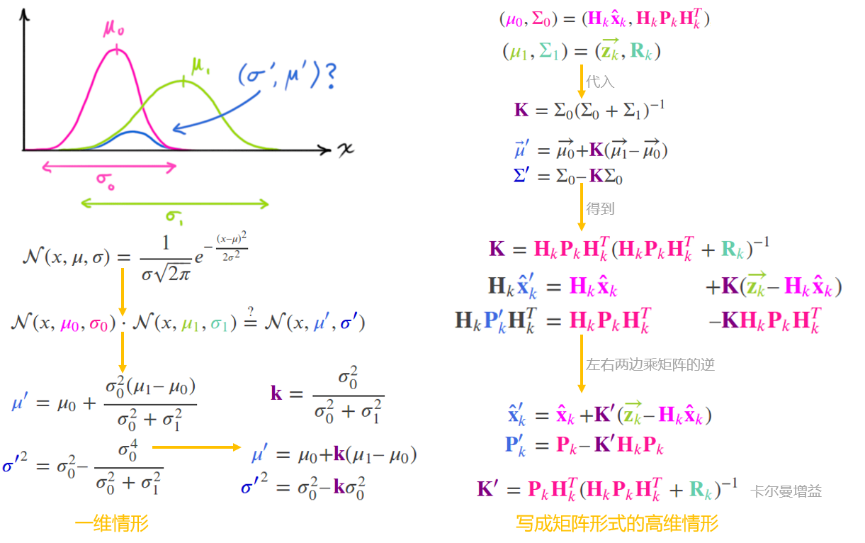
• 在实际应用中会对状态协方差矩阵 P 做一些微调，调整后的公式如下：
  $$\{\begin{array}{l}S=H{P}^{\prime }{H}^T+R\\ K=P^{\prime }{H}^T{S}^{-1}\\ y=z-H{x}^{\prime }\\ x=x^{\prime }+Ky\\ P=P^{\prime }-KS{K}^T=P^{\prime }-P^{\prime }{H}^T{S}^{-1}S{K}^T=P^{\prime }-P^{\prime }{H}^T{K}^T\end{array}$$

三、PaddleDetection/DeepSort 卡尔曼滤波代码实践

• kalman_filter.py 实现可参考： https://github.com/PaddlePaddle/PaddleDetection/tree/release/2.7/ppdet/modeling/mot/motion/kalman_filter.py
• 在目标跟踪的过程中我们主要估计 track 的两个重要的状态（包含位置和速度状态）：均值， 协方差
  • 均值：主要表示目标的 位置和速度 信息，由 bbox 的中心坐标、宽高比 w/h、高以及各自的速度变化值组成，即 $[c_x,c_y,r,h,v_x,v_y,v_r,v_h]$, 各个速度初始化为 0
  • 协方差：不仅包含了各个变量自己的不确定程度，还描述了它们之间的相关性（正相关，两个变量趋向于同时增大或减小；负相关，一个变量增大时，另一个变量减小），由上述的 8 个因素对应组成的 8*8 的对角矩阵，矩阵中数字越大则表明不确定性越大

# demo, 用于调试
import numpy as np
import kalman_filter as kf1

conf = 0.8
measurement = np.array([32, 56, 1.07, 126])

# 卡尔曼滤波器类初始化（状态转移矩阵 F：8*8 和 状态到观测的变换矩阵 4*8）
kf = kf1.KalmanFilter()

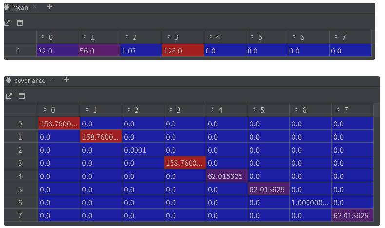
# 根据观测值初始化状态（mean, 8）与状态协方差（convariance, 8*8）：Create track from unassociated measurement
# var 为状态协方差矩阵（变量自身的变异程度及各个状态变量间的相互关系，初始化为 0，后续会不断变化)
mean, var = kf.initiate(measurement)

# 根据上一时刻状态进行预测和变换
mean, var = kf.predict(mean, var)

# 使用当前时刻传感器的测量值来更新最优估计值
mean, var = kf.update(mean, var, measurement, conf)

measurement1 = np.array([52, 36, 1.0, 66])
mean, var = kf.predict(mean, var)
mean, var = kf.update(mean, var, measurement1, conf)

measurement2 = np.array([66, 88, 1.1, 88])
mean, var = kf.predict(mean, var)
mean, var = kf.update(mean, var, measurement2, conf)
print(mean)

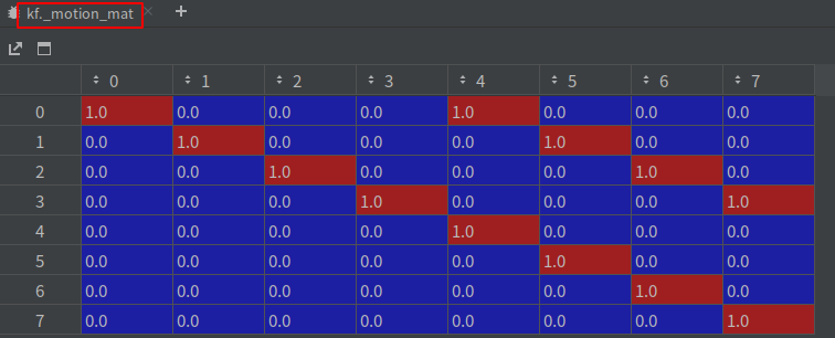
3.1、类初始化：__init__

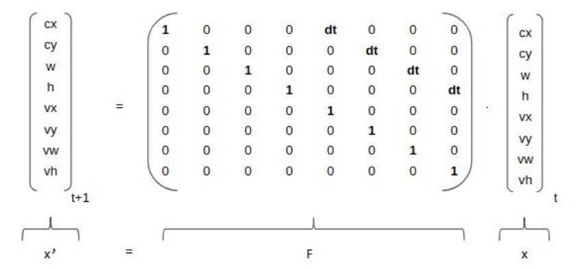
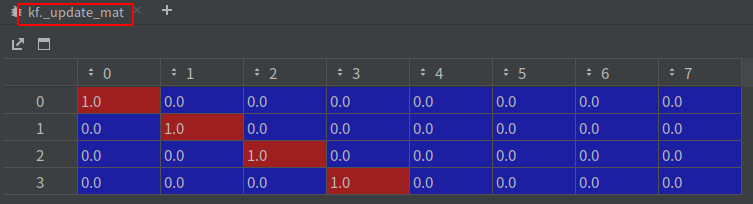
• 初始化卡尔曼对象时会有一个状态转移矩阵 F（_motion_mat 8*8） 和 状态到观测的变换矩阵 H（_update_mat 4*8），F 和 H 是不变的，dt 均为 1

class KalmanFilter(object):
    """
    A simple Kalman filter for tracking bounding boxes in image space.

    The 8-dimensional state space

        x, y, a, h, vx, vy, va, vh

    contains the bounding box center position (x, y), aspect ratio a, height h,
    and their respective velocities.

    Object motion follows a constant velocity model. The bounding box location
    (x, y, a, h) is taken as direct observation of the state space (linear
    observation model).

    """

    def __init__(self):
        ndim, dt = 4, 1.

        # Create Kalman filter model matrices
        # 状态转移矩阵 F：8×8 的单位矩阵，dt 置为 1
        self._motion_mat = np.eye(2 * ndim, 2 * ndim)
        for i in range(ndim):
            # 状态转移矩阵，8*8，ndim+i 代表各自的速度, dt=1 可以认为是一帧帧来做的
            self._motion_mat[i, ndim + i] = dt

        # 状态到观测的变换矩阵 H：4×8 的单位矩阵
        self._update_mat = np.eye(ndim, 2 * ndim)

        # Motion and observation uncertainty are chosen relative to the current
        # state estimate. These weights control the amount of uncertainty in
        # the model. This is a bit hacky.
        self._std_weight_position = 1. / 20
        self._std_weight_velocity = 1. / 160

---

3.2、根据观测值初始化状态（mean）与状态协方差（convariance）：initiate

• 均值和方差为每个 track 的属性，所以在构建新的 track 之前，需要 根据观测值 初始化其均值和协方差，在更新的过程中不断变化
• 均值 mean（对应推导公式中的 x, 8）：$mean=[c_x,c_y,r,h,0,0,0,0]$，分别表示中心点、宽高比、高及各自的速度变化，各个速度值初始化为 0
• 协方差 covariance（对应推导公式中的 P, 8*8）：表示目标位置信息和速度的不确定性，由 8*8 的对角矩阵表示，矩阵中数字越大表示不确定性越大
  • a. 首先，生成 1x8 的标准差 std=[h/10, h/10, 0.01, h/10, h/16, h/16. 0.0001, h/16]，根据目标高度生成（可能高度 h 代表性较强，高度越小就越远，高度越大就越近；当前位置（可以有多个目标）和宽高比（不怎么变，std 中给的值也比较小）代表性没那么强）
  • b. 其次，生成方差，np.square(std)
  • c. 最后，生成协方差，covariance = np.diag(np.square(std))

def initiate(self, measurement):
        """Create track from unassociated measurement.

        Parameters
        ----------
        measurement : ndarray
            Bounding box coordinates (x, y, a, h) with center position (x, y),
            aspect ratio a, and height h.

        Returns
        -------
        (ndarray, ndarray)
            Returns the mean vector (8 dimensional) and covariance matrix (8x8
            dimensional) of the new track. Unobserved velocities are initialized
            to 0 mean.

        """
        mean_pos = measurement               # (x, y, a, h)
        mean_vel = np.zeros_like(mean_pos)   # [0, 0, 0, 0], 刚出现的目标，认为其速度为 0
        mean = np.r_[mean_pos, mean_vel]     # [x, y, a, h, 0, 0, 0, 0]

        # 状态协方差矩阵 list len=8, 主要根据目标的高度构造方差矩阵
        # 根据目标高度生成（可能高度 h 代表性较强，高度越小就越远，高度越大就越近；
        # 当前位置（可以有多个目标）和宽高比（不怎么变，std 中给的值也比较小）代表性没那么强）
        std = [
            2 * self._std_weight_position * measurement[3],
            2 * self._std_weight_position * measurement[3],
            1e-2,
            2 * self._std_weight_position * measurement[3],
            10 * self._std_weight_velocity * measurement[3],
            10 * self._std_weight_velocity * measurement[3],
            1e-5,
            10 * self._std_weight_velocity * measurement[3]]  # 例如 std=[16.3, 16.3, 0.01, 16.3, 10.1875, 10.1875, 1e-05, 10.1875], list len=8
        
        # np.square(std)对std中的每个元素平方，np.diag 构成一个 8×8 的对角矩阵，对角线上的元素是 np.square(std)
        covariance = np.diag(np.square(std))
        
        return mean, covariance

---

3.3、根据上一时刻状态进行预测和变换：predict 和 project

3.3.1、predict: 根据上一时刻状态进行预测

• $x_t=F\ast x_{t-1}$，y, r, h 公式类似，dt 是当前帧和前一帧之间的差(程序中取值=1），将等号右边的矩阵乘法展开，可以得到
  • $c{x}_t=c{x}_{t-1}+v{x}_{t-1}$，新的位置=原来的位置+位移量；位移量=时间×速度，匀速模型
  • 程序实现代码为: mean = np.dot(mean, self._motion_mat.T)
  • 预测阶段：vx,vy,vw,vh 与上一帧一样，保持不变，更新阶段： vx,vy,vw,vh 发生变化，与上一帧不一样了
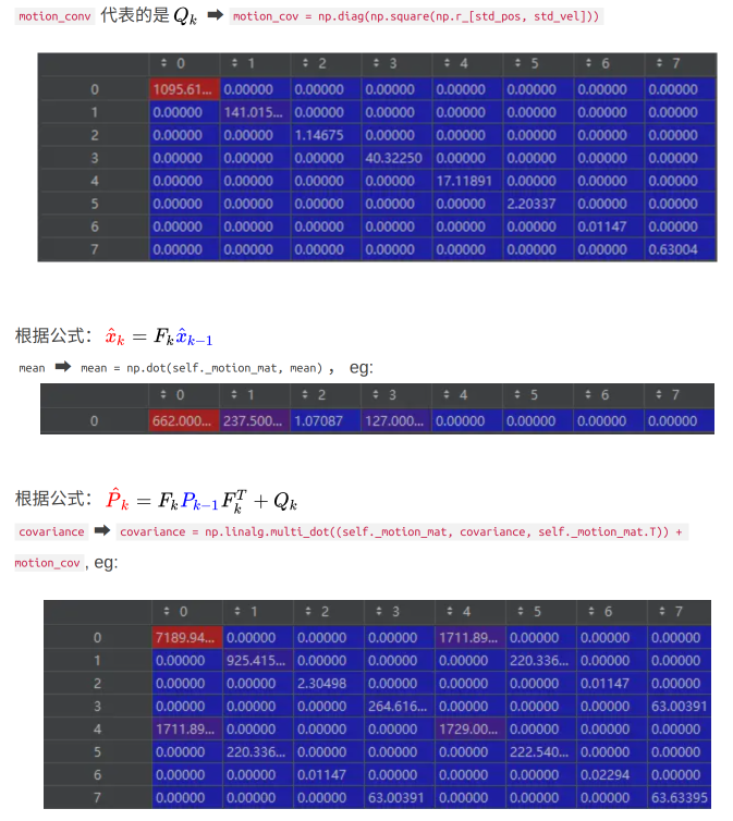
• $P_t=F{P}_{t-1}{F}^T+Q$， 预测噪声协方差矩阵 Q（motion_cov 8*8） 是变化的，每次都是 根据检测目标高生成的，与状态协方差矩阵生成方式类似（权重不同，是状态协方差矩阵的一半）
  

def predict(self, mean, covariance):
        """Run Kalman filter prediction step.

        Parameters
        ----------
        mean : ndarray
            The 8 dimensional mean vector of the object state at the previous
            time step.
        covariance : ndarray
            The 8x8 dimensional covariance matrix of the object state at the
            previous time step.

        Returns
        -------
        (ndarray, ndarray)
            Returns the mean vector and covariance matrix of the predicted
            state. Unobserved velocities are initialized to 0 mean.

        """
        # 预测噪声协方差矩阵 list len=8, 主要根据目标的高度构造方差矩阵
        # 根据目标高度生成（可能高度 h 代表性较强，高度越小就越远，高度越大就越近；
        # 当前位置（可以有多个目标）和宽高比（不怎么变，std 中给的值也比较小）代表性没那么强）
        std_pos = [
            self._std_weight_position * mean[3],
            self._std_weight_position * mean[3],
            1e-2,
            self._std_weight_position * mean[3]]
        std_vel = [
            self._std_weight_velocity * mean[3],
            self._std_weight_velocity * mean[3],
            1e-5,
            self._std_weight_velocity * mean[3]]

        # 预测噪声协方差矩阵 Q
        motion_cov = np.diag(np.square(np.r_[std_pos, std_vel]))

        #mean = np.dot(self._motion_mat, mean)
        mean = np.dot(mean, self._motion_mat.T)
        covariance = np.linalg.multi_dot((
            self._motion_mat, covariance, self._motion_mat.T)) + motion_cov

        return mean, covariance

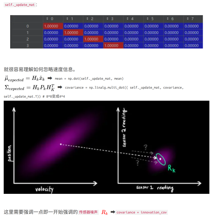
3.3.2、project: 状态到观测的变换

• 跟踪的空间向量与传感器向量空间不一致，需要借助投射矩阵将其转换在同一个向量空间
• 例如在我们跟踪的向量空间不仅包含目标的位置也包含其速度变化，但是在传感器向量空间是没有的（即目标检测仅仅输出目标的位置，没有输出目标运动的速度信息），需要进行转换 将速度信息忽略

# 创新点：加入 detection bbox 的得分参数 confidence 来控制传感器的噪声协方差矩阵 R（4*4，和观测高度 h 相关）
def project(self, mean, covariance, confidence=.0):
        """Project state distribution to measurement space.

        Parameters
        ----------
        mean : ndarray
            The state's mean vector (8 dimensional array).
        covariance : ndarray
            The state's covariance matrix (8x8 dimensional).
        confidence: 检测框置信度
        Returns
        -------
        (ndarray, ndarray)
            Returns the projected mean and covariance matrix of the given state
            estimate.

        """
        std = [
            self._std_weight_position * mean[3],
            self._std_weight_position * mean[3],
            1e-1,
            self._std_weight_position * mean[3]]
        
        # https://github.com/dyhBUPT/StrongSORT/blob/968848035c603732ad66a7cc8711a7b5b622f814/deep_sort/kalman_filter.py#L148-L149
        std = [(1 - confidence) * x for x in std]  # StrongSort NSA，创新点：根据观测的置信度调整传感器观测噪声 R

        # 传感器噪声 R 4*4，和观测高度 h 相关
        innovation_cov = np.diag(np.square(std))

        # 将均值向量映射到检测空间，由于测量矩阵 H 是一个 4X8 的单位矩阵，所以就相当于提取前4个位置向量[cx, cy, r, h] 8 位变 4 位
        mean = np.dot(self._update_mat, mean)
        covariance = np.linalg.multi_dot((
            self._update_mat, covariance, self._update_mat.T))   # 8*8 变成 4*4
        
        return mean, covariance + innovation_cov

# mean project
H=[[1. 0. 0. 0. 0. 0. 0. 0.]
   [0. 1. 0. 0. 0. 0. 0. 0.]
   [0. 0. 1. 0. 0. 0. 0. 0.]
   [0. 0. 0. 1. 0. 0. 0. 0.]]

Hx=[[1. 0. 0. 0. 0. 0. 0. 0.]
   [0. 1. 0. 0. 0. 0. 0. 0.]
   [0. 0. 1. 0. 0. 0. 0. 0.]
   [0. 0. 0. 1. 0. 0. 0. 0.]]*[cx,cy,r,h,vx,vy,vr,vh].^T
=[cx,cy,r,h]

---

3.4、使用当前时刻传感器的测量值来更新最优估计值：update

• 当对 track 匹配成功之后，需要根据匹配到的检测结果对其状态变量进行更新
• 基于当前 t 时刻检测到的 detection，校正与其关联的 track 的状态，得到一个更精确的结果，公式如下：
  $$\{\begin{array}{l}S=H{P}^{\prime }{H}^T+R\\ K=P^{\prime }{H}^T{S}^{-1}\\ y=z-H{x}^{\prime }\\ x=x^{\prime }+Ky\\ P=P^{\prime }-KH{K}^T\end{array}$$
• projected_cov 即为推导公式里面的 S (已经加上了观测噪声协方差矩阵)： $S=H{P}^{\prime }{H}^T+R$

def update(self, mean, covariance, measurement, confidence=.0):
        """Run Kalman filter correction step.

        Parameters
        ----------
        mean : ndarray
            The predicted state's mean vector (8 dimensional).
        covariance : ndarray
            The state's covariance matrix (8x8 dimensional).
        measurement : ndarray
            The 4 dimensional measurement vector (x, y, a, h), where (x, y)
            is the center position, a the aspect ratio, and h the height of the
            bounding box.
        confidence: 检测框置信度
        Returns
        -------
        (ndarray, ndarray)
            Returns the measurement-corrected state distribution.

        """
        # 1、将 mean, covariance 映射到检测空间（跟踪的空间向量与传感器向量空间转换），得到 Hx'（4，） 和 S （4，4） 
        # projected_mean=H*mean,测量矩阵H是一个4×8的单位矩阵，作用就是把1×8的均值向量提取出了前面的4个位置向量[cx,cy,r,h] 
        projected_mean, projected_cov = self.project(mean, covariance, confidence)
        
        # 2、通过 Cholesky 分解来加速逆矩阵 projected_cov^{-1} 的计算，得到 S^-1
        # chol_factor（4，4）, lower（True）
        chol_factor, lower = scipy.linalg.cho_factor(projected_cov, lower=True, check_finite=False)

        # 3、计算卡尔曼增益 K=P'*H^T*S^-1 (8, 4)
        kalman_gain = scipy.linalg.cho_solve((chol_factor, lower), 
                                             np.dot(covariance, self._update_mat.T).T, 
                                             check_finite=False).T
        
        # 4、计算 detection 和 track 的均值误差 y=z-Hx', 
        # z 为 detection 的均值向量，不包含速度变化值，即 z=[cx,cy,r,h],
        # H 称为测量矩阵，它将 track 的均值向量 x'映射到检测空间，该公式计算 detection 和 track 的均值误差
        innovation = measurement - projected_mean
        
        # 5、更新均值和方差
        # 新的均值向量(8,) x=x'+Ky=x'+k(z-Hx')
        # 新的协方差向量(8,8) P=P'-KHK^T
        new_mean = mean + np.dot(innovation, kalman_gain.T)
        new_covariance = covariance - np.linalg.multi_dot((kalman_gain, projected_cov, kalman_gain.T))
        
        return new_mean, new_covariance

---

3.5、基于卡尔曼滤波器的预测结果和观测值计算：gating_distance

• 卡尔曼预测的均值和方差的作用（需要先进行空间变换），体现在门函数中，计算 马氏距离

   def gating_distance(self, mean, covariance, measurements,
                        only_position=False, metric='maha'):
        """Compute gating distance between state distribution and measurements.
        A suitable distance threshold can be obtained from `chi2inv95`. If
        `only_position` is False, the chi-square distribution has 4 degrees of
        freedom, otherwise 2.
        Parameters
        ----------
        mean : ndarray
            Mean vector over the state distribution (8 dimensional).
        covariance : ndarray
            Covariance of the state distribution (8x8 dimensional).
        measurements : ndarray
            An Nx4 dimensional matrix of N measurements, each in
            format (x, y, a, h) where (x, y) is the bounding box center
            position, a the aspect ratio, and h the height.
        only_position : Optional[bool]
            If True, distance computation is done with respect to the bounding
            box center position only.
        Returns
        -------
        ndarray
            Returns an array of length N, where the i-th element contains the
            squared Mahalanobis distance between (mean, covariance) and
            `measurements[i]`.
        """
        mean, covariance = self.project(mean, covariance)
        if only_position:
            mean, covariance = mean[:2], covariance[:2, :2]
            measurements = measurements[:, :2]

        d = measurements - mean
        if metric == 'gaussian':
            return np.sum(d * d, axis=1)
        elif metric == 'maha':
            cholesky_factor = np.linalg.cholesky(covariance)
            z = scipy.linalg.solve_triangular(
                cholesky_factor, d.T, lower=True, check_finite=False,
                overwrite_b=True)
            squared_maha = np.sum(z * z, axis=0)
            return squared_maha
        else:
            raise ValueError('invalid distance metric')

---

四、FilterPy 卡尔曼滤波库简介

FilterPy 是一个实现了各种滤波器的 Python 模块（卡尔曼滤波和粒子滤波器），我们可以直接调用该库完成卡尔曼滤波器实现，其中的主要模块包括：

• filterpy.kalman：该模块主要实现了各种卡尔曼滤波器，包括常见的线性卡尔曼滤波器，扩展卡尔曼滤波器等
• filterpy.common：该模块主要提供支持实现滤波的各种辅助函数，其中计算噪声矩阵的函数，线性方程离散化的函数等
• filterpy.stats：该模块提供与滤波相关的统计函数，包括多元高斯算法，对数似然算法，PDF及协方差等
• filterpy.monte_carlo：该模块提供了马尔科夫链蒙特卡洛算法，主要用于粒子滤波

# 1、初始化: 状态变量维度、观测变量维度、状态变量、协方差矩阵、噪声矩阵、状态转移矩阵、状态到观测的变换矩阵
def __init__(self, dim_x, dim_z, dim_u = 0, x = None, P = None,
             Q = None, B = None, F = None, H = None, R = None):
    """Kalman Filter
        Refer to http:/github.com/rlabbe/filterpy

        Method
        -----------------------------------------
         Predict        |        Update
        -----------------------------------------
                        |  K = PH^T(HPH^T + R)^-1
        x = Fx + Bu     |  y = z - Hx
        P = FPF^T + Q   |  x = x + Ky
                        |  P = (1 - KH)P
                        |  S = HPH^T + R
        -----------------------------------------
        note: In update unit, here is a more numerically stable way: P = (I-KH)P(I-KH)' + KRK'

        Parameters
        ----------
        dim_x: int，状态变量维度
            dims of state variables, eg:(x,y,vx,vy)->4
        dim_z: int，观测变量维度
            dims of observation variables, eg:(x,y)->2
        dim_u: int，状态控制向量维度
            dims of control variables,eg: a->1
            p = p + vt + 0.5at^2
            v = v + at
            =>[p;v] = [1,t;0,1][p;v] + [0.5t^2;t]a
        """

    assert dim_x >= 1, 'dim_x must be 1 or greater'
    assert dim_z >= 1, 'dim_z must be 1 or greater'
    assert dim_u >= 0, 'dim_u must be 0 or greater'

    self.dim_x = dim_x
    self.dim_z = dim_z
    self.dim_u = dim_u

    # predict 相关变量初始化
    self.x = np.zeros((dim_x, 1)) if x is None else x      # state
    self.P = np.eye(dim_x)  if P is None else P            # uncertainty covariance
    self.Q = np.eye(dim_x)  if Q is None else Q            # process uncertainty for prediction
    self.B = None if B is None else B                      # control transition matrix
    self.F = np.eye(dim_x)  if F is None else F            # state transition matrix

    # update 相关变量初始化
    self.H = np.zeros((dim_z, dim_x)) if H is None else H  # Measurement function z=Hx
    self.R = np.eye(dim_z)  if R is None else R            # observation uncertainty
    self._alpha_sq = 1.                                    # fading memory control
    self.z = np.array([[None] * self.dim_z]).T             # observation
    self.K = np.zeros((dim_x, dim_z))                      # kalman gain
    self.y = np.zeros((dim_z, 1))                          # estimation error
    self.S = np.zeros((dim_z, dim_z))                      # system uncertainty, S = HPH^T + R
    self.SI = np.zeros((dim_z, dim_z))                     # inverse system uncertainty, SI = S^-1

    self.inv = np.linalg.inv
    self._mahalanobis = None                         # Mahalanobis distance of measurement
    self.latest_state = 'init'                       # last process name



# 2、predict：为了保证通用性，引入了遗忘系数 α，其作用在于调节对过往信息的依赖程度，α 越大对历史信息的依赖越小
def predict(self, u = None, B = None, F = None, Q = None):
    """
    Predict next state (prior) using the Kalman filter state propagation equations:
                         x = Fx + Bu
                         P = fading_memory*FPF^T + Q

    Parameters
    ----------

    u : ndarray
        Optional control vector. If not `None`, it is multiplied by B
        to create the control input into the system.

    B : ndarray of (dim_x, dim_z), or None
        Optional control transition matrix; a value of None
        will cause the filter to use `self.B`.

    F : ndarray of (dim_x, dim_x), or None
        Optional state transition matrix; a value of None
        will cause the filter to use `self.F`.

    Q : ndarray of (dim_x, dim_x), scalar, or None
        Optional process noise matrix; a value of None will cause the
        filter to use `self.Q`.
    """

    if B is None:
        B = self.B
    if F is None:
        F = self.F
    if Q is None:
        Q = self.Q
    elif np.isscalar(Q):
        Q = np.eye(self.dim_x) * Q

    # x = Fx + Bu
    if B is not None and u is not None:
        self.x = F @ self.x + B @ u
    else:
        self.x = F @ self.x

    # P = fading_memory*FPF' + Q
    self.P = self._alpha_sq * (F @ self.P @ F.T) + Q
    self.latest_state = 'predict'


# 3、update, 不断迭代的系统变量，分别是系统的状态 x、协方差矩阵 P 和卡尔曼增益 K
def update(self, z, R = None, H = None):
    """
    Update Process, add a new measurement (z) to the Kalman filter.
                K = PH^T(HPH^T + R)^-1
                y = z - Hx
                x = x + Ky
                P = (I - KH)P or P = (I-KH)P(I-KH)' + KRK'

    If z is None, nothing is computed.

    Parameters
    ----------
    z : (dim_z, 1): array_like
        measurement for this update. z can be a scalar if dim_z is 1,
        otherwise it must be convertible to a column vector.

    R : ndarray, scalar, or None
        Optionally provide R to override the measurement noise for this
        one call, otherwise  self.R will be used.

    H : ndarray, or None
        Optionally provide H to override the measurement function for this
        one call, otherwise self.H will be used.
    """

    if z is None:
        self.z = np.array([[None] * self.dim_z]).T
        self.y = np.zeros((self.dim_z, 1))
        return

    z = reshape_z(z, self.dim_z, self.x.ndim)

    if R is None:
        R = self.R
    elif np.isscalar(R):
        R = np.eye(self.dim_z) * R

    if H is None:
        H = self.H

    if self.latest_state == 'predict':
        # common subexpression for speed
        PHT = self.P @ H.T

        # S = HPH' + R
        # project system uncertainty into measurement space
        self.S = H @ PHT + R

        self.SI = self.inv(self.S)


        # K = PH'inv(S)
        # map system uncertainty into kalman gain
        self.K = PHT @ self.SI

        # P = (I-KH)P(I-KH)' + KRK'
        # This is more numerically stable and works for non-optimal K vs
        # the equation P = (I-KH)P usually seen in the literature.
        I_KH = np.eye(self.dim_x) - self.K @ H
        self.P = I_KH @ self.P @ I_KH.T + self.K @ R @ self.K.T


    # y = z - Hx
    # error (residual) between measurement and prediction
    self.y = z - H @ self.x

    self._mahalanobis = math.sqrt(float(self.y.T @ self.SI @ self.y))

    # x = x + Ky
    # predict new x with residual scaled by the kalman gain

    self.x = self.x + self.K @ self.y
    self.latest_state = 'update'

• 卡尔曼滤波器中进行运动估计时使用的候选框表示形式为 [x, y, s, r]，其中 x,y 为中心点坐标，s 为面积，r 为宽高比

import numpy as np

# 将候选框从左上右下坐标形式转换为中心点及面积坐标的形式
def convert_bbox_to_z(bbox):
    """
    将[x1,y1,x2,y2]形式的检测框转为滤波器的状态表示形式[x,y,s,r]。其中x，y是框的中心坐标，s是面积，尺度，r是宽高比
    :param bbox: [x1,y1,x2,y2] 分别是左上角坐标和右下角坐标
    :return: [ x, y, s, r ] 4行1列，其中x,y是box中心位置的坐标，s是面积，r是纵横比w/h
    """
    w = bbox[2] - bbox[0]
    h = bbox[3] - bbox[1]
    x = bbox[0] + w / 2.
    y = bbox[1] + h / 2.
    s = w * h
    r = w / float(h)
    return np.array([x, y, s, r]).reshape((4, 1))

# 将候选框从中心点及面积坐标的形式转换为左上右下坐标形式
def convert_x_to_bbox(x, score=None):
    """
    将[cx，cy，s，r]的目标框表示转为[x_min，y_min，x_max，y_max]的形式
    :param x:[ x, y, s, r ],其中x,y是box中心位置的坐标，s是面积，r
    :param score: 置信度
    :return:[x1,y1,x2,y2],左上角坐标和右下角坐标
    """
    w = np.sqrt(x[2] * x[3])
    h = x[2] / w
    if score is None:
        return np.array([x[0] - w / 2., x[1] - h / 2., x[0] + w / 2., x[1] + h / 2.]).reshape((1, 4))
    else:
        return np.array([x[0] - w / 2., x[1] - h / 2., x[0] + w / 2., x[1] + h / 2., score]).reshape((1, 5))

---

五、参考资料

1、目标跟踪（一）DeepSORT论文及代码分析
2、https://www.bzarg.com/p/how-a-kalman-filter-works-in-pictures/#more-491
3、详解卡尔曼滤波原理
4、卡尔曼滤波：从入门到精通
5、http:/github.com/rlabbe/filterpy
6、多目标跟踪（MOT）中的卡尔曼滤波（Kalman filter）和匈牙利(Hungarian)算法详解
7、详解 SORT 与卡尔曼滤波算法