


 本文介绍了如何使用BayesPrismR包和网页版工具对bulkRNA-seq数据进行细胞类型和状态的反卷积分析,包括数据准备、质量控制、异常基因过滤、构建Prism对象、运行Prism和结果提取与可视化。该方法适用于整合bulk和单细胞RNA测序数据的肿瘤学研究。
官方网站:BayesPrism Gateway
参考文献:Chu, T., Wang, Z., Pe’er, D. Danko, C. G. Cell type and gene expression deconvolution with BayesPrism enables Bayesian integrative analysis across bulk and single-cell RNA sequencing in oncology. Nat Cancer 3, 505–517 (2022). Cell type and gene expression deconvolution with BayesPrism enables Bayesian integrative analysis across bulk and single-cell RNA sequencing in oncology | Nature Cancer
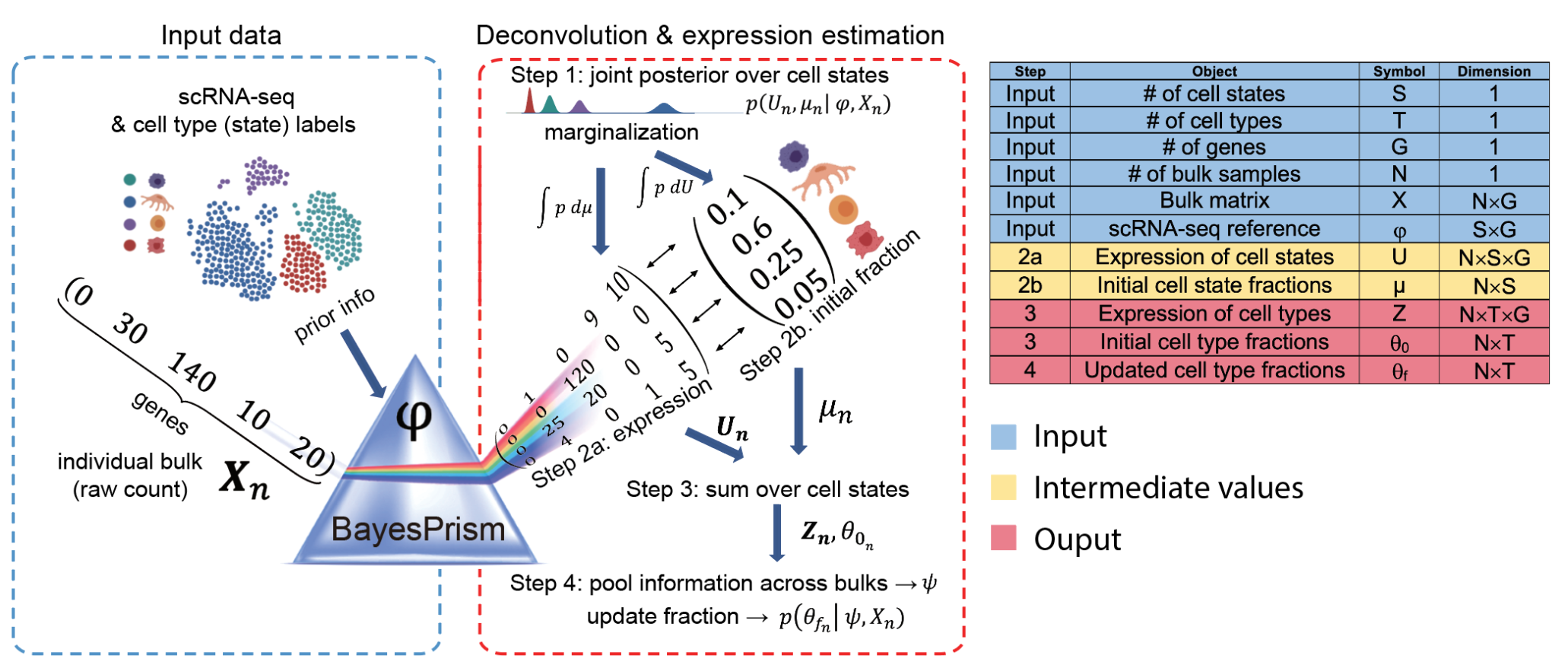
BayesPrism反卷积算法流程。
最近在学习怎么给bulkRNA数据分群,看到了这个R包,按照官方网站的流程,这两天使用了一下,是可以做出来的。不过我也看到它还出了网页版的,不用写代码,只需上传实验数据就可以得到结果,感兴趣的可以去官网试试。
一、安装BayesPrism并加载
library(devtools)
install_github("Danko-Lab/BayesPrism/BayesPrism")
library(BayesPrism)
二、数据准备
需要准备四个数据:
1.bk.dat:bulk RNA-seq 原始计数矩阵(官方建议使用非标准化和未转换的计数矩阵)。rownames是样本ID,colnames是基因名称/ID。
2.sc.dat:scRNA-seq 原始计数矩阵。rownames是细胞ID,colnames是基因名称/ID。
注意:bk.dat和sc.dat的基因名称/ID需要保持一致。
3.cell.type.labels:字符向量,长度与nrow(sc.dat)相同,表示sc.dat中每个细胞的类型。
4.cell.state.labels:表示sc.dat中每个细胞的亚类型。
这里说明一下cell.type.labels和cell.state.labels的区别,拿我的参考sc.dat(心脏scRNA)来说,心脏细胞可以分为Fibroblast、Endothelial、Ventricular Cardiomyocyte、Atrial Cardiomyocyte等几种细胞类型,每个细胞都会被分为这些细胞类型之一,这就是cell.type.labels。将这些细胞类型继续细分,可以分为更细的亚群,例如Fibroblast1、Fibroblast2、Fibroblast3等,这就是cell.state.labels。
(说明:我的参考数据集sc.dat来源于https://doi.org/10.1038/s41586-020-2797-4)
#load sc.dat
load(file = "sc.dat.RData")
#如果参考单细胞数据集是seurat格式,可以提取counts
#sc.dat <- sc[["RNA"]]@counts
dim(sc.dat)#查看 sc.dat
# [1] 14000 33538
head(rownames(sc.dat))#细胞id
#[1] "AAACCCAAGAACGCGT-1-H0015_apex" "AACCCAATCCGTGTAA-1-H0015_apex"
#[3] "AACGTCATCGGCCCAA-1-H0015_apex" "AAGACAAGTGCCCTTT-1-H0015_apex"
#[5] "AAGATAGGTTAAGACA-1-H0015_apex" "AAGGAATCATCATTTC-1-H0015_apex"
head(colnames(sc.dat))#基因名/ID
#[1] "MIR1302-2HG" "FAM138A"     "OR4F5"       "AL627309.1"  "AL627309.3"
#[6] "AL627309.2"
#load bk.dat 原始矩阵(最好未标准化)
load(file = "bk.dat.RData")
dim(bk.dat)
# [1] 6 19536
head(rownames(bk.dat))#样本id
#[1] "PAS.1" "PAS.3" "PAS.4" "PAS.5" "PAS.6" "PAS.7"
head(colnames(bk.dat))#基因名/ID
#[1] "WASH7P" "RP11-34P13.15" "RP11-34P13.13" "WASH9P"
#[5] "RP4-669L17.4" "RP11-206L10.17"#load cell.type.labels
#可以从参考单细胞数据集提取或者直接load
#从参考单细胞数据集提取
cell.type.labels <- sc@meta.data[["cell_type"]]
#直接load
#load(file = "cell.type.label.RData")
sort(table(cell.type.labels))
#cell.type.labels
# doublets Mesothelial
# 16 19
# Neuronal Adipocytes
# 100 109
# Lymphoid Smooth_muscle_cells
# 428 499
# Myeloid Atrial_Cardiomyocyte
# 609 672
# NotAssigned Fibroblast
# 1041 1835
# Endothelial Pericytes
# 2153 2413
#Ventricular_Cardiomyocyte
# 4106 #load cell.state.labels
#可以从参考单细胞数据集提取或者直接load
#从参考单细胞数据集提取
cell.state.labels <- sc@meta.data[["cell_states"]]
#直接load
#load(file = "cell.type.state.RData")
sort(table(cell.state.labels))
#cell.state.labels
# IL17RA+Mo NC6 NC4 NØ aCM5
# 0 1 2 2 2
# NC5 Adip3 Adip4 NC3 EC9_FB-like
# 3 5 7 8 11
# NC2 vCM5 doublets EC8_ln Meso
# 12 15 16 18 19
# Adip2 FB7 MØ_AgP DC MØ_mod
# 20 23 23 27 29
# B_cells CD4+T_tem NKT CD14+Mo aCM4
# 31 31 38 42 42
# FB6 LYVE1+MØ3 Mo_pi DOCK4+MØ2 LYVE1+MØ2
# 44 44 47 51 52
# Mast EC10_CMC-like LYVE1+MØ1 CD4+T_cytox NC1
# 60 65 70 72 74
# CD8+T_cytox NK Adip1 CD8+T_tem PC4_CMC-like
# 75 76 77 78 79
# FB5 DOCK4+MØ1 CD16+Mo SMC2_art aCM3
# 80 94 95 98 120
# EC4_immune EC7_atria aCM2 FB4 FB3
# 129 129 140 185 225
# EC6_ven vCM4 EC2_cap EC3_cap PC2_atria
# 231 252 317 347 365
# aCM1 EC5_art PC3_str SMC1_basic FB2
# 368 376 379 401 416
# EC1_cap vCM3 vCM2 FB1 nan
# 530 622 798 862 1041
# PC1_vent vCM1
# 1590 2419
#查看cell.type.labels和cell.state.labels的关系
table(cbind.data.frame(cell.state.labels,cell.type.labels))三、细胞类型和状态的质量控制
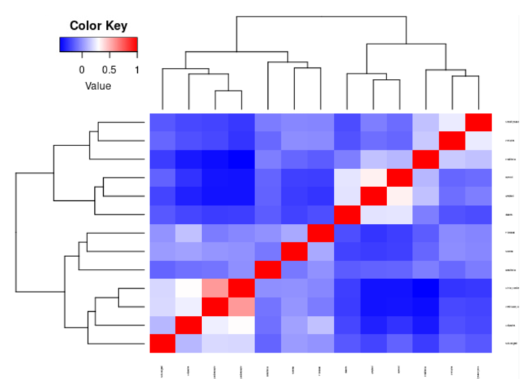
作者建议首先绘制细胞状态之间和细胞类型之间的相关矩阵。如果types/states没有足够的信息量,则低质量的types/states往往聚集在一起。使用者可以以更高的分辨率重新聚类数据,或者将这些types/states与最相似的types/states合并。如果重新聚类和合并不适用,也可以删除它们。一般来说如果参考数据集是已发表文章里的数据,问题都不大。
plot.cor.phi (input=sc.dat,
                         input.labels=cell.state.labels,
                         title="cell state correlation",
                         #specify pdf.prefix if need to output to pdf
                         #pdf.prefix="gbm.cor.cs",
                         cexRow=0.2, cexCol=0.2,
                         margins=c(2,2))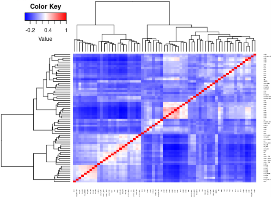
plot.cor.phi (input=sc.dat,
                         input.labels=cell.type.labels,
                         title="cell type correlation",
                         #specify pdf.prefix if need to output to pdf
                         #pdf.prefix="gbm.cor.ct",
                         cexRow=0.5, cexCol=0.5,
                         )
四、过滤异常基因
#单细胞数据的离群基因
sc.stat <- plot.scRNA.outlier(
  input=sc.dat, #make sure the colnames are gene symbol or ENSMEBL ID
  cell.type.labels=cell.type.labels,
  species="hs", #currently only human(hs) and mouse(mm) annotations are supported
  return.raw=TRUE #return the data used for plotting.
  #pdf.prefix="gbm.sc.stat" specify pdf.prefix if need to output to pdf
)
head(sc.stat)#查看
#            exp.mean.log   max.spec other_Rb  chrM  chrX  chrY    Rb
#MIR1302-2HG    -18.42068 0.07692308    FALSE FALSE FALSE FALSE FALSE
#FAM138A        -18.42068 0.07692308    FALSE FALSE FALSE FALSE FALSE
#OR4F5          -18.42068 0.07692308    FALSE FALSE FALSE FALSE FALSE
#AL627309.1     -11.88445 0.34987702    FALSE FALSE FALSE FALSE FALSE
#AL627309.3     -18.42068 0.07692308    FALSE FALSE FALSE FALSE FALSE
#AL627309.2     -17.35768 0.68115362    FALSE FALSE FALSE FALSE FALSE
#              Mrp   act    hb MALAT1
#MIR1302-2HG FALSE FALSE FALSE  FALSE
#FAM138A     FALSE FALSE FALSE  FALSE
#OR4F5       FALSE FALSE FALSE  FALSE
#AL627309.1  FALSE FALSE FALSE  FALSE
#AL627309.3  FALSE FALSE FALSE  FALSE
#AL627309.2  FALSE FALSE FALSE  FALSE
#bulk数据的离群基因
bk.stat <- plot.bulk.outlier(
  bulk.input=bk.dat,#make sure the colnames are gene symbol or ENSMEBL ID
    sc.input=sc.dat, #make sure the colnames are gene symbol or ENSMEBL ID
  cell.type.labels=cell.type.labels,
  species="hs", #currently only human(hs) and mouse(mm) annotations are supported
  return.raw=TRUE
  #pdf.prefix="gbm.bk.stat" specify pdf.prefix if need to output to pdf
)
#> EMSEMBLE IDs detected.
head(bk.stat)#查看
#               exp.mean.log max.spec other_Rb  chrM  chrX  chrY    Rb
#WASH7P            -12.35343       NA    FALSE FALSE FALSE FALSE FALSE
#RP11.34P13.15     -14.67106       NA    FALSE FALSE FALSE FALSE FALSE
#RP11.34P13.13     -15.75896       NA    FALSE FALSE FALSE FALSE FALSE
#WASH9P            -12.36118       NA    FALSE FALSE FALSE FALSE FALSE
#RP4.669L17.4      -15.73036       NA    FALSE FALSE FALSE FALSE FALSE
#RP11.206L10.17    -16.60104       NA    FALSE FALSE FALSE FALSE FALSE
#                 Mrp   act    hb MALAT1
#WASH7P         FALSE FALSE FALSE  FALSE
#RP11.34P13.15  FALSE FALSE FALSE  FALSE
#RP11.34P13.13  FALSE FALSE FALSE  FALSE
#WASH9P         FALSE FALSE FALSE  FALSE
#RP4.669L17.4   FALSE FALSE FALSE  FALSE
#RP11.206L10.17 FALSE FALSE FALSE  FALSE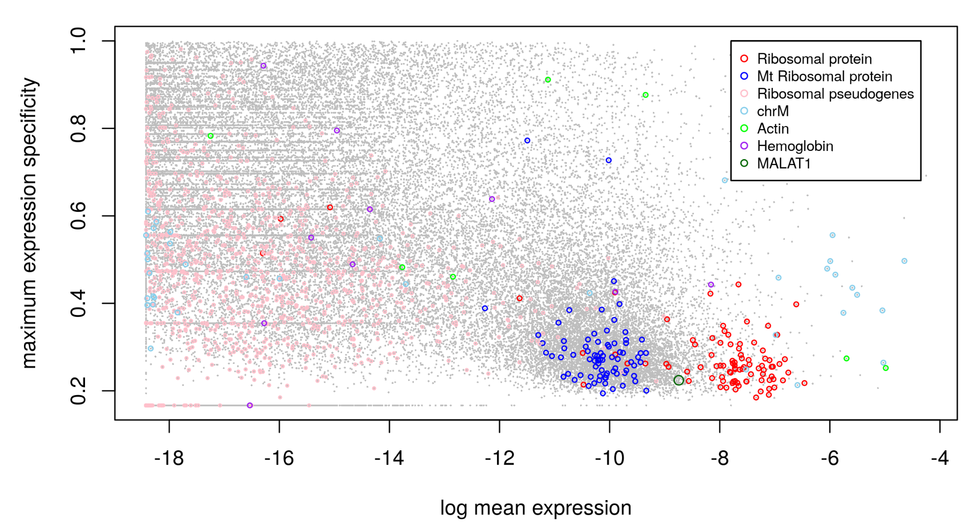
#过滤异常基因
sc.dat.filtered <- cleanup.genes (input=sc.dat,
                                  input.type="count.matrix",
                                    species="hs",
                                    gene.group=c( "Rb","Mrp","other_Rb","chrM","MALAT1","chrX","chrY","hb","act"),
                                    exp.cells=5)
#> EMSEMBLE IDs detected.
#> number of genes filtered in each category:
#>       Rb      Mrp other_Rb     chrM   MALAT1     chrX     chrY
#>       89       78     1011       37        1     2464      594
#> A total of  4214  genes from Rb Mrp other_Rb chrM MALAT1 chrX chrY  have been excluded
#> A total of  24343  gene expressed in fewer than  5  cells have been excluded
#检查不同类型基因表达的一致性
plot.bulk.vs.sc (sc.input = sc.dat.filtered,
bulk.input = bk.dat
#pdf.prefix="gbm.bk.vs.sc" specify pdf.prefix if need to output to pdf
)
#选择相关性最高的组别
sc.dat.filtered.pc <- select.gene.type (sc.dat.filtered,
gene.type = "protein_coding")
#protein_coding
#15421 
除了可以根据相关性选择,还可以根据marker genes选择,后续构建prism对象时,修改reference=sc.dat.filtered.sig即可。
# Select marker genes (Optional)
# performing pair-wise t test for cell states from different cell types

diff.exp.stat <- get.exp.stat(sc.dat=sc.dat[,colSums(sc.dat>0)>3],# filter genes to reduce memory use
                                          cell.type.labels=cell.type.labels,
                                          cell.state.labels=cell.state.labels,
                                          psuedo.count=0.1, #a numeric value used for log2 transformation. =0.1 for 10x data, =10 for smart-seq. Default=0.1.
                                          cell.count.cutoff=50, # a numeric value to exclude cell state with number of cells fewer than this value for t test. Default=50.
                                          n.cores=1 #number of threads
                                          )
sc.dat.filtered.pc.sig <- select.marker (sc.dat=sc.dat.filtered.pc,
stat=diff.exp.stat,
pval.max=0.01,
lfc.min=0.1)
#> number of markers selected for each cell type:
#> tumor : 8686
#> myeloid : 575
#> pericyte : 114
#> endothelial : 244
#> tcell : 123
#> oligo : 86
dim(sc.dat.filtered.pc.sig)
#> [1] 23793 7874五、构建Prism 对象
myPrism <- new.prism(
  reference=sc.dat.filtered.pc,
  mixture=bk.dat,
  input.type="count.matrix",
  cell.type.labels = cell.type.labels,
  cell.state.labels = cell.state.labels,
  key=NULL,#
  outlier.cut=0.01,
  outlier.fraction=0.1,
)
#> Number of outlier genes filtered from mixture = 6
#> Aligning reference and mixture...
#> Nornalizing reference...
六、运行Prism
bp.res <- run.prism(prism = myPrism, n.cores=50)
bp.res#结果
slotNames(bp.res)
#[1] "prism"                       "posterior.initial.cellState"
#[3] "posterior.initial.cellType"  "reference.update"
#[5] "posterior.theta_f"           "control_param"
save(bp.res, file="bp.res.rdata")
七、提取结果
#提取细胞类型
theta <- get.fraction(bp=bp.res,
                       which.theta="final",
                       state.or.type="type")

head(theta)
#Smooth_muscle_cells Fibroblast Ventricular_Cardiomyocyte Pericytes
#PAS.1        8.848475e-02 0.08555898              1.308257e-06 0.1528725
#PAS.3        7.484271e-02 0.05720185              2.233524e-01 0.1996966
#PAS.4        2.099285e-01 0.24647069              1.713629e-06 0.1081544
#PAS.5        1.977008e-05 0.05069060              1.603388e-01 0.2419610
#PAS.6        6.157566e-06 0.08187859              1.745477e-01 0.3104268
#PAS.7        3.874839e-03 0.04515391              5.437359e-01 0.1819701
#       NotAssigned Endothelial     Myeloid     Neuronal   Adipocytes
#PAS.1 7.303103e-07   0.1831999 0.015510885 2.813086e-03 0.0148733471
#PAS.3 4.898819e-06   0.2158705 0.027300737 7.452442e-04 0.0454755292
#PAS.4 1.268937e-04   0.2931470 0.045910484 4.554966e-03 0.0114139200
#PAS.5 7.329211e-03   0.4364701 0.004353618 7.092140e-05 0.0195800954
#PAS.6 1.118299e-02   0.3421726 0.009172048 2.602303e-03 0.0063014147
#PAS.7 1.311456e-06   0.1511986 0.011427483 4.775924e-07 0.0006889955
#      Atrial_Cardiomyocyte     Lymphoid     doublets  Mesothelial
#PAS.1          0.434162035 2.178387e-02 5.817286e-07 7.380315e-04
#PAS.3          0.124304008 2.897200e-02 7.336232e-05 2.160056e-03
#PAS.4          0.005265647 7.391574e-02 9.497520e-07 1.109058e-03
#PAS.5          0.076649524 1.258866e-06 2.534140e-03 1.007315e-06
#PAS.6          0.058374551 2.760672e-04 3.033184e-03 2.559008e-05
#PAS.7          0.050493620 1.126307e-02 7.747565e-07 1.909557e-04
write.csv(theta,file="theta.csv")

#提取变异系数
theta.cv <- bp.res@posterior.theta_f@theta.cv
head(theta.cv)

#extract posterior mean of cell type-specific gene expression count matrix Z
#Z.tumor <- get.exp (bp=bp.res,
#                    state.or.type="type",
#                    cell.name="tumor")

#head(t(Z.tumor[1:5,]))
八、可视化
上一步得到的theta其实就是细胞类型的比例,画个图看一下。
ratio <- as.data.frame(theta)
ratio <- t(ratio)
ratio <- as.data.frame(ratio)
ratio <- tibble::rownames_to_column(ratio)
ratio <- melt(ratio)
colourCount = length(ratio$rowname)
ggplot(ratio) +
  geom_bar(aes(x = variable,y = value,fill = rowname),stat = "identity",width = 0.7,size = 0.5,colour = '#222222')+
  theme_classic() +
  labs(x='Sample',y = 'Ratio')+
  coord_flip()+
  theme(panel.border = element_rect(fill=NA,color="black", size=0.5, linetype="solid"))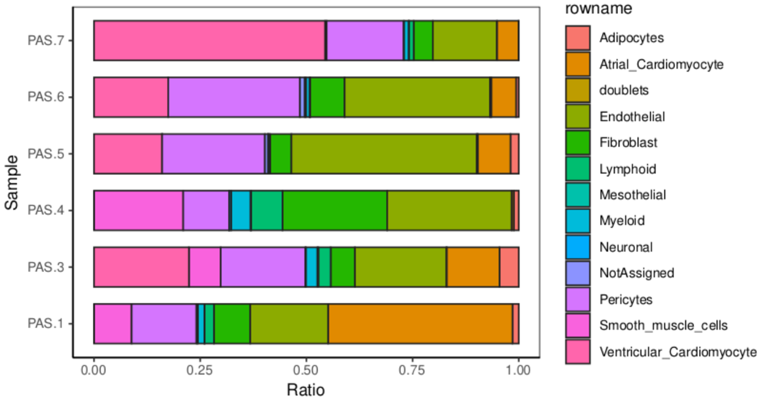
以上就是BayesPrism的使用方法,我对BayesPrism的算法没有深入了解,感兴趣的可以看看原论文,其他问题欢迎交流~


 4613
4613

 被折叠的 条评论
为什么被折叠?
被折叠的 条评论
为什么被折叠?
 到【灌水乐园】发言


