SCS【41】基于贝叶斯反卷积法整合分析bulk和scRNA-seq (BayesPrism)

最新推荐文章于 2024-06-24 21:24:26 发布

桓峰基因

最新推荐文章于 2024-06-24 21:24:26 发布

阅读量914

点赞数 24

文章标签：计算机视觉人工智能机器学习

本文链接：https://blog.csdn.net/weixin_41368414/article/details/137488736

版权

‍

简介

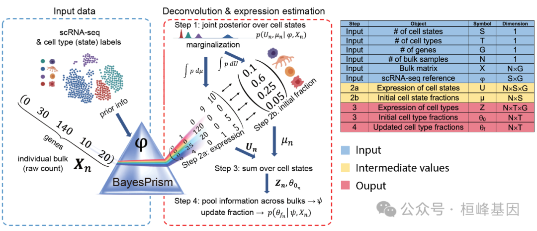
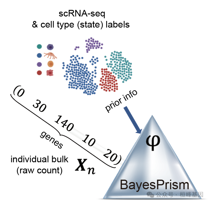
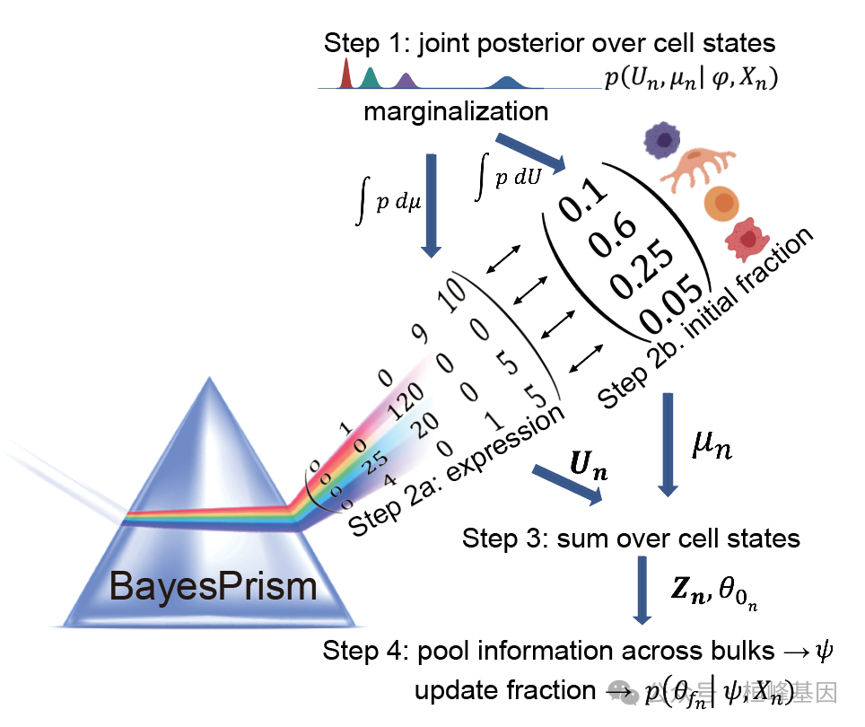
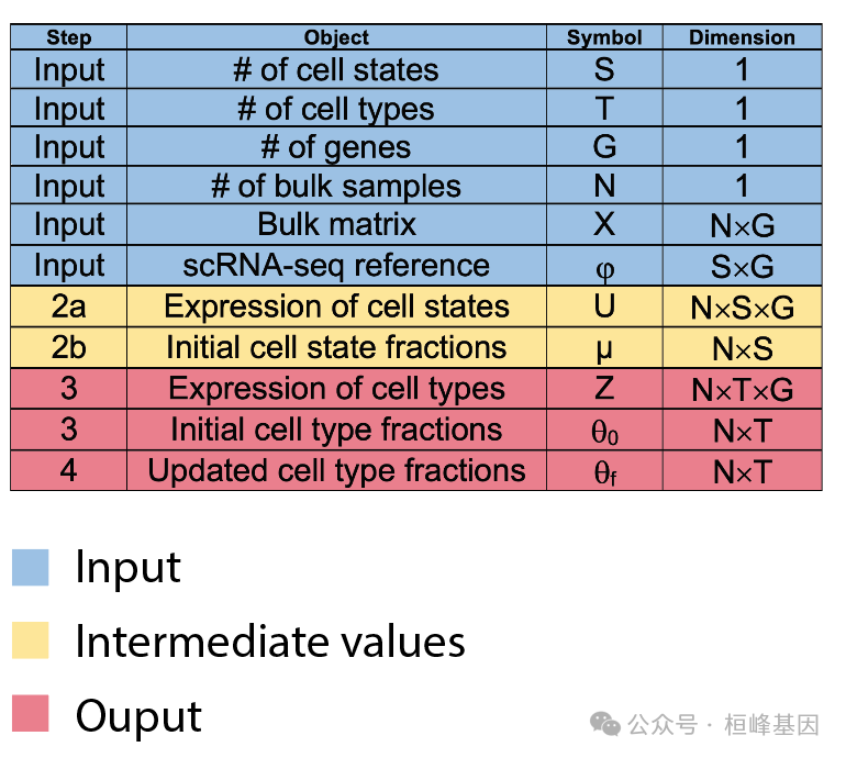
BayesPrism 使用从匹配或相似组织类型收集的scRNA-seq样本，对大量RNA-seq(和空间转录组学)进行细胞类型和基因表达反褶积。将scRNA-seq作为先验信息，估计P(θ,Z|X,ϕ)，即细胞类型分数θ和细胞类型特异性基因表达Z在每个群体中的联合后验分布，条件是参考ϕ和每个观察群体X。

软件包安装

library("devtools");
install_github("Danko-Lab/BayesPrism/BayesPrism")

数据读取

使用BayesPrism对大量RNA-seq数据集TCGA-GBM进行反卷积，使用Yuan等人从8个保留队列中收集的scRNA-seq数据集。

rdata文件包含运行BayesPrism所需的四个对象：

bk.dat:批量RNA-seq表达的样本按基因原始计数矩阵。行名是样本id，而列名是基因名。

sc.dat:单细胞RNA-seq表达的细胞-基因原始计数矩阵。行名是细胞id，而列名是基因名。data应该是一个矩阵。如果您的sc.dat是一个稀疏矩阵(dgCMatrix)，则应该将其转换为密集矩阵。

cell.type.labels:是一个与nrow(sc.dat)长度相同的字符向量，用于表示引用中每个细胞类型。

cell.state.labels:是一个与nrow(sc.dat)长度相同的字符向量，用于表示引用中每个细胞的细胞状态。在我们的例子中，通过对每个患者的恶性细胞进行亚聚类来获得恶性细胞的细胞状态，通过对所有患者的髓细胞进行聚类来获得髓细胞的细胞状态。为这两种细胞类型定义了多个细胞状态，因为包含大量异质性，同时也有足够数量的细胞用于亚聚类。

library(BayesPrism)
source("run_gibbs.R")
load("BayesPrism-main/tutorial.dat/tutorial.gbm.rdata")
ls()
## [1] "bk.dat"            "cell.state.labels" "cell.type.labels" 
## [4] "run.gibbs.refPhi"  "sc.dat"
dim(bk.dat)
## [1]   169 60483
head(rownames(bk.dat))
## [1] "TCGA-06-2563-01A-01R-1849-01" "TCGA-06-0749-01A-01R-1849-01"
## [3] "TCGA-06-5418-01A-01R-1849-01" "TCGA-06-0211-01B-01R-1849-01"
## [5] "TCGA-19-2625-01A-01R-1850-01" "TCGA-19-4065-02A-11R-2005-01"
head(colnames(bk.dat))
## [1] "ENSG00000000003.13" "ENSG00000000005.5"  "ENSG00000000419.11"
## [4] "ENSG00000000457.12" "ENSG00000000460.15" "ENSG00000000938.11"

dim(sc.dat)
## [1] 23793 60294
head(rownames(sc.dat))
## [1] "PJ016.V3" "PJ016.V4" "PJ016.V5" "PJ016.V6" "PJ016.V7" "PJ016.V8"
head(colnames(sc.dat))
## [1] "ENSG00000130876.10" "ENSG00000134438.9"  "ENSG00000269696.1" 
## [4] "ENSG00000230393.1"  "ENSG00000266744.1"  "ENSG00000202281.1"

sort(table(cell.type.labels))
## cell.type.labels
##       tcell       oligo    pericyte endothelial     myeloid       tumor 
##          67         160         489         492        2505       20080
sort(table(cell.state.labels))
## cell.state.labels
## PJ017-tumor-6 PJ032-tumor-5     myeloid_8 PJ032-tumor-4 PJ032-tumor-3 
##            22            41            49            57            62 
table(cbind.data.frame(cell.state.labels, cell.type.labels))
##                  cell.type.labels
## cell.state.labels endothelial myeloid oligo pericyte tcell tumor
##     endothelial           492       0     0        0     0     0
##     myeloid_0               0     550     0        0     0     0
##     myeloid_1               0     526     0        0     0     0
##     myeloid_2               0     386     0        0     0     0
##     oligo                   0       0   160        0     0     0
##     pericyte                0       0     0      489     0     0
##     PJ016-tumor-0           0       0     0        0     0   621
##     PJ016-tumor-1           0       0     0        0     0   619
##     tcell                   0       0     0        0    67     0

实例操作

细胞类型和状态的质量控制

首先绘制细胞状态和细胞类型之间的两两相关矩阵，了解其的质量情况。在细胞类型/状态没有足够数量的信息表示的情况下(低细胞计数和/或低库大小)，低质量的细胞类型/状态倾向于聚集在一起。可以以更高的粒度重新聚类数据，或者将这些细胞类型/状态与最相似的细胞类型/状态合并，或者删除。

细胞状态统计

##QC of cell type and state labels
plot.cor.phi (input=sc.dat,
              input.labels=cell.state.labels,
              title="cell state correlation",
              #specify pdf.prefix if need to output to pdf
              #pdf.prefix="gbm.cor.cs", 
              cexRow=0.2, cexCol=0.2,
              margins=c(2,2))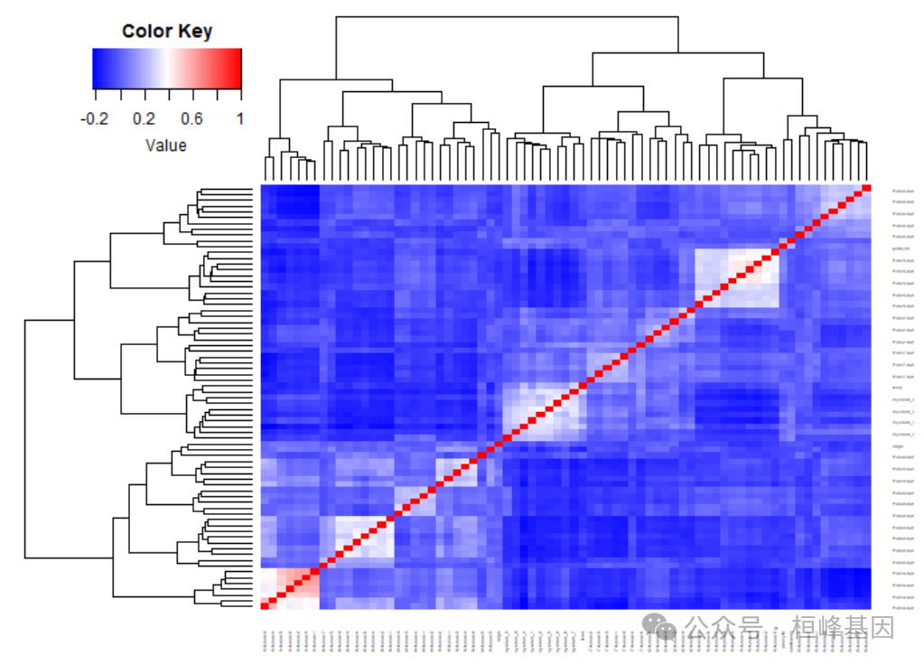

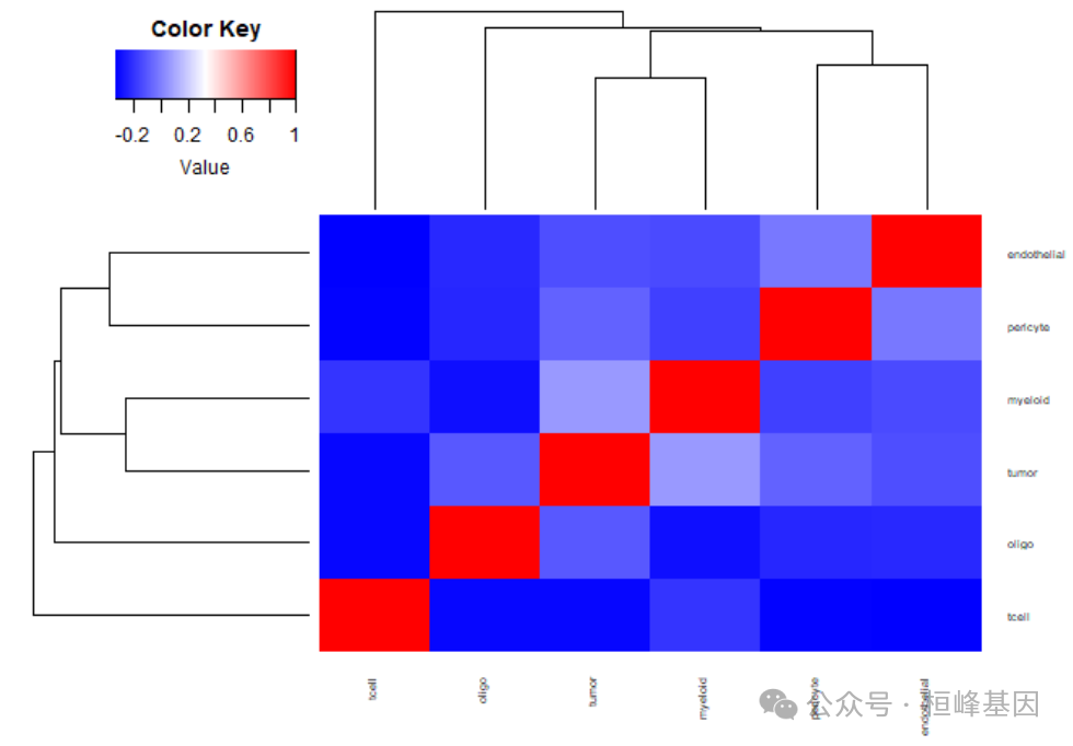
细胞类型统计

plot.cor.phi (input=sc.dat, 
              input.labels=cell.type.labels, 
              title="cell type correlation",
              #specify pdf.prefix if need to output to pdf
              #pdf.prefix="gbm.cor.ct",
              cexRow=0.5, cexCol=0.5,
)

过滤异常基因

核糖体蛋白基因和线粒体基因等表达量较大的基因可能在分布中占主导地位，并对推断产生偏差。这些基因通常不能提供区分细胞类型的信息，而且可能是大量虚假变异的来源。因此，不利于反褶积，建议去除这些基因。

可视化从scRNA-seq参考的异常基因的分布。计算每个基因在所有细胞类型中的平均表达量和细胞类型特异性评分。

可视化和确定scRNA-seq数据中的异常基因

如图所示，核糖体蛋白基因通常表现出高平均表达和低细胞类型特异性评分。

sc.stat <- plot.scRNA.outlier(
  input=sc.dat, #make sure the colnames are gene symbol or ENSMEBL ID 
  cell.type.labels=cell.type.labels,
  species="hs", #currently only human(hs) and mouse(mm) annotations are supported
  return.raw=TRUE #return the data used for plotting. 
  #pdf.prefix="gbm.sc.stat" specify pdf.prefix if need to output to pdf
)
## EMSEMBLE IDs detected.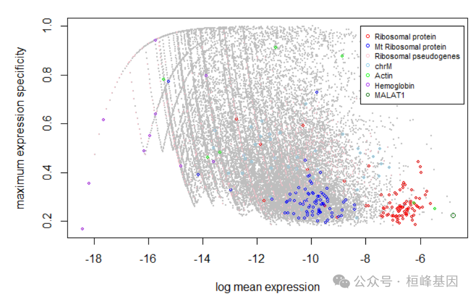

如果需要，用户还可以根据该功能输出的统计数据从sc.dat中提取基因子集。

sc.stat显示了每个基因的归一化平均表达量(x轴)和最大特异性(y轴)的对数，以及每个基因是否属于潜在的异常值类别。other_Rb是一组主要由核糖体伪基因组成的调控基因。同样，也可以从大量RNA-seq中看到异常基因。我们计算每个基因在所有细胞类型中的平均表达量。由于没有从大量数据中获得细胞类型水平信息，因此从scRNA-seq中计算细胞类型特异性评分，如上所述。在大量RNA-seq中可视化异常基因。

bk.stat <- plot.bulk.outlier(
  bulk.input=bk.dat,#make sure the colnames are gene symbol or ENSMEBL ID 
  sc.input=sc.dat, #make sure the colnames are gene symbol or ENSMEBL ID 
  cell.type.labels=cell.type.labels,
  species="hs", #currently only human(hs) and mouse(mm) annotations are supported
  return.raw=TRUE
  #pdf.prefix="gbm.bk.stat" specify pdf.prefix if need to output to pdf
)
## EMSEMBLE IDs detected.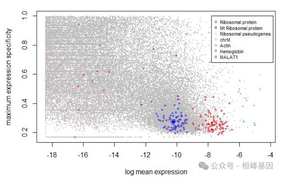

过滤scRNA-seq数据中的异常基因

接下来，从选定的群体中移除基因。注意，当参考基因和混合基因的性别不相同时，建议排除来自chrX和chrY的基因。我们也去除转录较低的基因，因为这些基因的转录测量容易产生噪声。去除这些基因也可以加快计算速度。

### Filter outlier genes from scRNA-seq data
sc.dat.filtered <- cleanup.genes(input = sc.dat, input.type = "count.matrix", species = "hs",
    gene.group = c("Rb", "Mrp", "other_Rb", "chrM", "MALAT1", "chrX", "chrY"), exp.cells = 5)
## EMSEMBLE IDs detected.
## number of genes filtered in each category: 
##       Rb      Mrp other_Rb     chrM   MALAT1     chrX     chrY 
##       89       78     1011       37        1     2464      594 
## A total of  4214  genes from Rb Mrp other_Rb chrM MALAT1 chrX chrY  have been excluded 
## A total of  24343  gene expressed in fewer than  5  cells have been excluded
dim(sc.dat.filtered)
## [1] 23793 31737

接下来，检查不同类型基因的基因表达的一致性。由于bulk和单细胞数据通常由不同的实验方案收集，可能对不同类型的基因具有不同的敏感性。

#note this function only works for human data. For other species, you are advised to make plots by yourself.
plot.bulk.vs.sc (sc.input = sc.dat.filtered,
                 bulk.input = bk.dat
                 #pdf.prefix="gbm.bk.vs.sc" specify pdf.prefix if need to output to pdf
)
## EMSEMBLE IDs detected.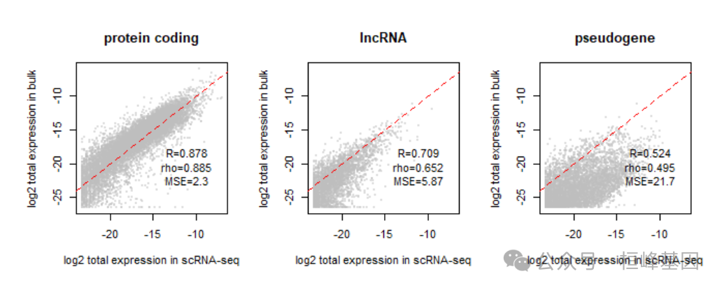

蛋白质编码基因是最一致的组之间的两个分析。为了减少批量效应和加快计算速度，对蛋白质编码基因进行了反卷积。尝试在所有基因上运行 BayesPrism，结果是相似的。

sc.dat.filtered.pc <- select.gene.type(sc.dat.filtered, gene.type = "protein_coding")
## EMSEMBLE IDs detected.
## number of genes retained in each category: 
## 
## protein_coding 
##          16148

提供了一个选择基因的功能，通过在不同细胞类型的细胞状态之间使用成对t检验进行差异表达。

diff.exp.stat <- get.exp.stat(sc.dat=sc.dat[,colSums(sc.dat>0)>3],# filter genes to reduce memory use
                              cell.type.labels=cell.type.labels,
                              cell.state.labels=cell.state.labels,
                              pseudo.count=0.1, #a numeric value used for log2 transformation. =0.1 for 10x data, =10 for smart-seq. Default=0.1.
                              cell.count.cutoff=50, # a numeric value to exclude cell state with number of cells fewer than this value for t test. Default=50.
                              n.cores=1 #number of threads
)

要将计数矩阵置于特征基因之上，可以如下方式：

sc.dat.filtered.pc.sig <- select.marker(sc.dat = sc.dat.filtered.pc, stat = diff.exp.stat,
    pval.max = 0.01, lfc.min = 0.1)
## number of markers selected for each cell type: 
## tumor :  8686 
## myeloid :  575 
## pericyte :  114 
## endothelial :  244 
## tcell :  123 
## oligo :  86

构造 prism 对象

prism 对象包含运行 BayesPrism 所需的所有数据，即scRNA-seq参考矩阵，每行参考的细胞类型和细胞状态标签，以及批量RNA-seq的混合矩阵。

当使用scRNA-seq计数矩阵作为输入(推荐)时，用户需要指定输入。Type = "count.matrix"。输入的另一个选项类型是“GEP”(基因表达谱)，这是一种由基因基质构成的细胞状态。当使用来自其他分析的参考时，例如已排序的批量数据时，使用此选项。

参数key是cell.type.labels中的一个字符，对应于恶性细胞类型。如果没有恶性细胞，或者参比和混合物之间的恶性细胞来自匹配的样本，则设置为NULL，在这种情况下，所有细胞类型将被平等对待。

## Construct a prism object.
myPrism <- new.prism(reference = sc.dat.filtered.pc, mixture = bk.dat, input.type = "count.matrix",
    cell.type.labels = cell.type.labels, cell.state.labels = cell.state.labels, key = "tumor",
    outlier.cut = 0.01, outlier.fraction = 0.1, )
## number of cells in each cell state 
## cell.state.labels
## PJ017-tumor-6 PJ032-tumor-5     myeloid_8 PJ032-tumor-4 PJ032-tumor-3 
##            22            41            49            57            62 
## Number of outlier genes filtered from mixture = 6 
## Aligning reference and mixture... 
## Normalizing reference...

运行 BayesPrism

控制Gibbs 采样和优化的参数可以使用 gibbs.control 和 opt.control。

bp.res <- run.prism(prism = myPrism, n.cores=16)
#Run Gibbs sampling using updated reference ... 
#Current time:  2024-04-07 11:11:44.384737 
#Estimated time to complete:  22mins 
#Estimated finishing time:  2024-04-07 11:33:00.384737 
#Start run... 
#snowfall 1.84-6.3 initialized (using snow 0.4-4): parallel execution on 16 CPUs.

结果说明

BayesPrism 预计会产生以下结果:

使用函数从run.prism的输出中提取反卷积的细胞类型分数和表达。

# saveRDS(bp.res,file = 'bp.res.rds') #保存 rds
bp.res <- readRDS("bp.res.rds")  # 读取 rd
slotNames(bp.res)
## [1] "prism"                       "posterior.initial.cellState"
## [3] "posterior.initial.cellType"  "reference.update"           
## [5] "posterior.theta_f"           "control_param"
theta <- get.fraction(bp = bp.res, which.theta = "final", state.or.type = "type")

细胞类型分数提取变异系数(CV)

theta.cv <- bp.res@posterior.theta_f@theta.cv

head(theta.cv)
##                                     tumor      myeloid     pericyte endothelial
## TCGA-06-2563-01A-01R-1849-01 0.0001853812 0.0017158155 0.0036206921 0.001541438
## TCGA-06-0749-01A-01R-1849-01 0.0002731345 0.0006926134 0.8350796062 0.005117005
## TCGA-06-5418-01A-01R-1849-01 0.0001498423 0.0008984021 0.0055755747 0.003166470
## TCGA-06-0211-01B-01R-1849-01 0.0001581423 0.0015382228 0.0052983068 0.001923780
## TCGA-19-2625-01A-01R-1850-01 0.0001466586 0.0022468948 0.0154427073 0.004493776
## TCGA-19-4065-02A-11R-2005-01 0.0002586784 0.0012542921 0.0009487042 0.004773946
##                                   tcell       oligo
## TCGA-06-2563-01A-01R-1849-01 0.04018182 0.007231069
## TCGA-06-0749-01A-01R-1849-01 1.03161517 0.001435592
## TCGA-06-5418-01A-01R-1849-01 1.21310651 0.010367026
## TCGA-06-0211-01B-01R-1849-01 0.88098343 0.494090752
## TCGA-19-2625-01A-01R-1850-01 0.60583812 0.008741805
## TCGA-19-4065-02A-11R-2005-01 0.05843119 0.002575675

theta.cv量化了后验分布的集中程度。较高的θ值与较低的CV相关。当执行排序统计时，例如Spearman的秩相关，当CV高于某个数字时，可能会屏蔽，例如>0.1. 较低的测序深度，如空间转录组学，通常与较高的CV相关。对Visium数据进行反卷积时，CV的合理截止值可能是~0.5。

# extract posterior mean of cell type-specific gene expression count matrix Z
Z.tumor <- get.exp(bp = bp.res, state.or.type = "type", cell.name = "tumor")

Reference

Tran, K.A., Addala, V., Johnston, R.L. et al. Performance of tumour microenvironment deconvolution methods in breast cancer using single-cell simulated bulk mixtures. Nat Commun 14, 5758 (2023). https://doi.org/10.1038/s41467-023-41385-5
Hippen, A.A., Omran, D.K., Weber, L.M. et al. Performance of computational algorithms to deconvolve heterogeneous bulk ovarian tumor tissue depends on experimental factors. Genome Biol 24, 239 (2023). https://doi.org/10.1186/s13059-023-03077-7
Hu, M., Chikina, M. Heterogeneous pseudobulk simulation enables realistic benchmarking of cell-type deconvolution methods. bioRxiv 2023.01.05.522919; doi: https://doi.org/10.1101/2023.01.05.522919

单细胞生信分析教程

Topic 6. 克隆进化之 Canopy

Topic 7. 克隆进化之 Cardelino

Topic 8. 克隆进化之 RobustClone

SCS【1】今天开启单细胞之旅，述说单细胞测序的前世今生

SCS【2】单细胞转录组之 cellranger

SCS【3】单细胞转录组数据 GEO 下载及读取

SCS【4】单细胞转录组数据可视化分析 (Seurat 4.0)

SCS【5】单细胞转录组数据可视化分析 (scater)

SCS【6】单细胞转录组之细胞类型自动注释 (SingleR)

SCS【7】单细胞转录组之轨迹分析 (Monocle 3) 聚类、分类和计数细胞

SCS【8】单细胞转录组之筛选标记基因 (Monocle 3)

SCS【9】单细胞转录组之构建细胞轨迹 (Monocle 3)

SCS【10】单细胞转录组之差异表达分析 (Monocle 3)

SCS【11】单细胞ATAC-seq 可视化分析 (Cicero)

SCS【12】单细胞转录组之评估不同单细胞亚群的分化潜能 (Cytotrace)

SCS【13】单细胞转录组之识别细胞对“基因集”的响应 (AUCell)

SCS【14】单细胞调节网络推理和聚类 (SCENIC)

SCS【15】细胞交互：受体-配体及其相互作用的细胞通讯数据库 (CellPhoneDB)

SCS【16】从肿瘤单细胞RNA-Seq数据中推断拷贝数变化 (inferCNV)

SCS【17】从单细胞转录组推断肿瘤的CNV和亚克隆 (copyKAT)

SCS【18】细胞交互：受体-配体及其相互作用的细胞通讯数据库 (iTALK)

SCS【19】单细胞自动注释细胞类型 (Symphony)

SCS【20】单细胞数据估计组织中细胞类型(Music)

SCS【21】单细胞空间转录组可视化 (Seurat V5)

SCS【22】单细胞转录组之 RNA 速度估计 (Velocyto.R)

SCS【23】单细胞转录组之数据整合 (Harmony)

SCS【24】单细胞数据量化代谢的计算方法 (scMetabolism)

SCS【25】单细胞细胞间通信第一部分细胞通讯可视化（CellChat）

SCS【26】单细胞细胞间通信第二部分通信网络的系统分析（CellChat）

SCS【27】单细胞转录组之识别标记基因（scran）

SCS【28】单细胞转录组加权基因共表达网络分析(hdWGCNA)

SCS【29】单细胞基因富集分析 (singleseqgset)

SCS【30】单细胞空间转录组学数据库(STOmics DB)

SCS【31】减少障碍，加速单细胞研究数据库(Single Cell PORTAL)

SCS【32】基于scRNA-seq数据中推断单细胞的eQTLs (eQTLsingle)

SCS【33】单细胞转录之全自动超快速的细胞类型鉴定 (ScType)

SCS【34】单细胞/T细胞/抗体免疫库数据分析(immunarch)

SCS【35】单细胞转录组之去除双细胞 (DoubletFinder)

SCS【36】单细胞转录组之k-近邻图差异丰度测试(miloR)

SCS【37】hdWGCNA在空间转录组学中的作用

SCS【38】单细胞转录组之免疫浸润分析(escape)

SCS【39】单细胞转录组之降维散点图的美化 (SCpubr)

SCS【40】单细胞转录组之便捷式细胞类型注释（scMayoMap）

号外号外，桓峰基因单细胞生信分析免费培训课程即将开始，快来报名吧！

桓峰基因，铸造成功的您！

未来桓峰基因公众号将不间断的推出单细胞系列生信分析教程，

敬请期待！！

桓峰基因官网正式上线，请大家多多关注，还有很多不足之处，大家多多指正！

http://www.kyohogene.com/

桓峰基因和投必得合作，文章润色优惠85折，需要文章润色的老师可以直接到网站输入领取桓峰基因专属优惠券码：KYOHOGENE，然后上传，付款时选择桓峰基因优惠券即可享受85折优惠哦！https://www.topeditsci.com/

‍

桓峰基因

关注

24
点赞
踩
26

收藏

觉得还不错? 一键收藏
0
评论
SCS【41】基于贝叶斯反卷积法整合分析bulk和scRNA-seq (BayesPrism)

‍‍简介BayesPrism 使用从匹配或相似组织类型收集的scRNA-seq样本，对大量RNA-seq(和空间转录组学)进行细胞类型和基因表达反褶积。将scRNA-seq作为先验信息，估计P(θ,Z|X,ϕ)，即细胞类型分数θ和细胞类型特异性基因表达Z在每个群体中的联合后验分布，条件是参考ϕ和每个观察群体X。软件包安装library("devtools");install_github("D...
复制链接

扫一扫