FOC控制中Clark/iClark和Park/iPark变换及matpoltlib仿真

注：本文部分内容及图片来自网络，如有侵权通知删除！

三相交流电：

• 三相交流电是由三个频率相同、电势振幅相等、相位差互差120°角的交流电路组成的电力系统。日常用电系统中的三相四线制中电压为380/220V，即线电压为380V；相电压则随接线方式而异：若使用星形接法，相电压为220v；三角形接法，相电压则为380V。
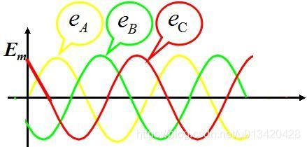
• 三相电压：每根相线（火线）与中性线(零线)间的电压叫相电压，其有效值用UA、UB、UC表示；相线间的电压叫线电压，其有 效值用UAB、UBC、UCA表示。因为三相交流电源的三个线圈产生的交流电压相位相差120°，三个线圈作星形连接时，线电压等于相电压的根号3倍。我们通常讲的电压是220伏，380伏，就是三相四线制供电时的相电压和线电压。我国日常电路中，相电压是220V，线电压是380V（380V≈√3*220V）。工程上，讨论三相电源电压大小时，通常指的是电源的线电压。如三相四线制电源电压380V，指的是线电压380V。三相发电机在并网发电时或用三相电驱动三相交流电动机时，必须考虑相序的问题，否则会引起重大事故，为了防止接线错误，低压配电线路中规定用颜色区分各相，黄色表示A相，绿色表示B相，红色表示C相。
  

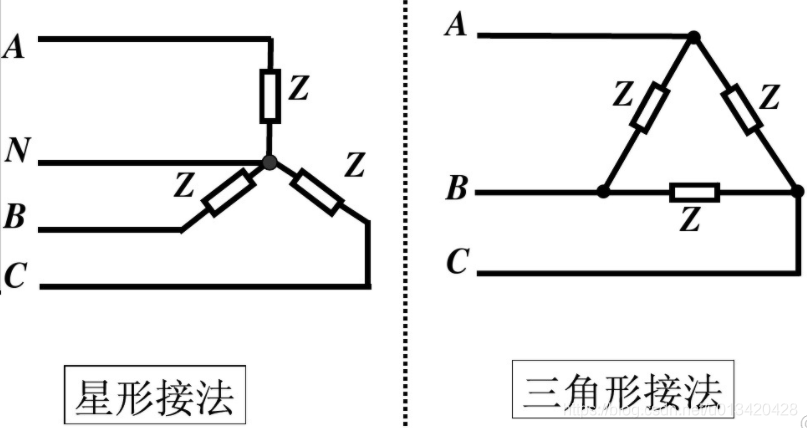
负载的两种接法（Y-型接法，Δ-型接法）

(电机正转-表达函数)：

$$\begin{array}{l}Ua=Vm\ast cos(\omega t)\\ Ub=Vm\ast cos(\omega t-\frac{2}{3}\pi )\\ Uc=Vm\ast cos(\omega t+\frac{2}{3}\pi )\end{array}$$

(电机反转-表达函数)：

$$\begin{array}{l}Ua=Vm\ast cos(\omega t)\\ Ub=Vm\ast cos(\omega t+\frac{2}{3}\pi )\\ Uc=Vm\ast cos(\omega t-\frac{2}{3}\pi )\end{array}$$
Vm:表示电压的幅度;
t:表示时间;
ω:角速度ω=Φ/t=2π/T=2πf,角速度等于2π除以周期，也等于2π乘以频率,其中：Φ角度, t时间, T周期, f频率, π圆周率;

根据公式可以看出，三相电压是随时间变化的正弦波，相位差120°，如下图所示：

FOC控制中,有两种坐标转换,分别是clark变换和park变换:

• clark变换将abc坐标系转换为αβ坐标系。
• park变换将静止的αβ坐标系转换为旋转的dq坐标系。
  逆变换：
• iclark变换将αβ坐标系转换为abc坐标系。
• ipark变换将旋转的dq坐标系转换为静止的αβ坐标系。

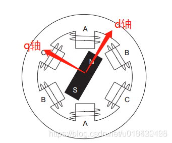
αβ坐标系：α轴β轴相位差90°，如下图所示：

dq坐标系：dq坐标相对于定子是旋转坐标系，相对转子是静止坐标系（dq坐标旋转的角速度和转子的旋转角速度相同）：

d轴方向与转子的磁链方向重和，又称为直轴；
q轴方向与转子的磁链方向垂直，又称为交轴；

电机功率P、转矩T、速度V 之间的关系:
功率=力·速度,表达公式：P=F·V
转矩(T)=扭力(F)·作用半径®, 推导出F=T/R
线速度(V)=2πR·每秒转速（n秒）
d轴:调节幅度(电机的转速);
q轴:调节相位(电机的转矩);

Clark Tranformation 3s-2s,clark转换公式：

$$\left[\begin{array}{c}U\alpha \\ U\beta \end{array}\right]=m\cdot \left|\begin{array}{ccc}Ua& -Ub\cdot cos(60°)& -Uc\cdot cos(60°)\\ 0& Ub\cdot cos(30°)& -Uc\cdot cos(30°)\end{array}\right|=m\cdot \left[\begin{array}{ccc}1& -\frac{1}{2}& -\frac{1}{2}\\ 0& \frac{\sqrt{(}3)}{2}& -\frac{\sqrt{(}3)}{2}\end{array}\right]\cdot \left[\begin{array}{c}Ua\\ Ub\\ Uc\end{array}\right]$$
矩阵展开：
$$\begin{array}{l}U\alpha =m\cdot (Ua-\frac{1}{2}\cdot Ub-\frac{1}{2}\cdot Uc)\\ U\beta =m\cdot (\frac{\sqrt{3}}{2}\cdot Ub-\frac{\sqrt{3}}{2}\cdot Uc)\end{array}$$
若m=√(2/3),变换前后，功率不变。又称为:Concordia变换。
若m=2/3,变换前后,幅值不变,恒幅值。
将m=2/3代入式中得：
$$\begin{array}{l}U\alpha =Ua\\ U\beta =\frac{1}{\sqrt{3}}\cdot (Ua+2\cdot Ub)\end{array}$$

# Inverse Clark Transformation 2s-3s, iClark逆变换:

$$\left[\begin{array}{c}Ua\\ Ub\\ Uc\end{array}\right]=m^{\prime }\cdot \left[\begin{array}{cc}1& 0\\ -\frac{1}{2}& \frac{\sqrt{3}}{2}\\ -\frac{1}{2}& -\frac{\sqrt{3}}{2}\end{array}\right]\cdot \left[\begin{array}{c}U\alpha \\ U\beta \end{array}\right]$$
矩阵展开：
$$\begin{array}{l}Ua=m^{\prime }\cdot (U\alpha )\\ Ub=m^{\prime }\cdot (-\frac{1}{2}\cdot U\alpha +\frac{\sqrt{3}}{2}\cdot U\beta )\\ Uc=m^{\prime }\cdot (-\frac{1}{2}\cdot U\alpha -\frac{\sqrt{3}}{2}\cdot U\beta )\end{array}$$
若m′=√(2/3),变换前后，功率不变。
若m′=1,变换前后,幅值不变。

Park Transformation 3s-3r,park转换：

$$\left[\begin{array}{c}Ud\\ Uq\\ U0\end{array}\right]=\frac{2}{3}\cdot \left[\begin{array}{ccc}cos(\theta )& cos(\theta -\frac{2}{3}\pi )& cos(\theta +\frac{2}{3}\pi )\\ -sin(\theta )& -sin(\theta -\frac{2}{3}\pi )& -sin(\theta +\frac{2}{3}\pi )\\ \frac{1}{2}& \frac{1}{2}& \frac{1}{2}\end{array}\right]\cdot \left[\begin{array}{c}Ua\\ Ub\\ Uc\end{array}\right]$$
$$\begin{gathered} Ud=U\alpha \cdot cos(\theta )+U\beta \cdot sin(\theta ) \\ Uq=U\beta \cdot cos(\theta )-U\alpha \cdot sin(\theta ) \\ or \\ Ud=U\alpha \cdot cos(\theta )+U\beta \cdot sin(\theta ) \\ Uq=-U\alpha \cdot sin(\theta )+U\beta \cdot cos(\theta ) \end{gathered}$$

inverse Park Tranformation 3r-3s,iPark逆转换:

$$\left[\begin{array}{c}Ua\\ Ub\\ Uc\end{array}\right]=\left[\begin{array}{ccc}cos(\theta )& -sin(\theta )& 1\\ cos(\theta -\frac{2}{3}\pi )& -sin(\theta -\frac{2}{3}\pi )& 1\\ cos(\theta +\frac{2}{3}\pi )& -sin(\theta +\frac{2}{3}\pi )& 1\end{array}\right]\cdot \left[\begin{array}{c}Ud\\ Uq\\ U0\end{array}\right]$$

$$\left[\begin{array}{c}U\alpha \\ U\beta \end{array}\right]=\left[\begin{array}{cc}cos(\theta )& -sin(\theta )\\ sin(\theta )& cos(\theta )\end{array}\right]\cdot \left[\begin{array}{c}Ud\\ Uq\end{array}\right]$$

相关变量值：

• π=180°(平角), 2π=360°(周角)，这里π表示弧度
• cos(60°) = 1/2 = 0.5
• cos(30°) = √3/2 ≈ 0.866025
• √3 = 1.7320508075688772935274463415059
• 2/3 = 0.66666666666666666666666666666667
• √(2/3) = 0.81649658092772603273242802490196

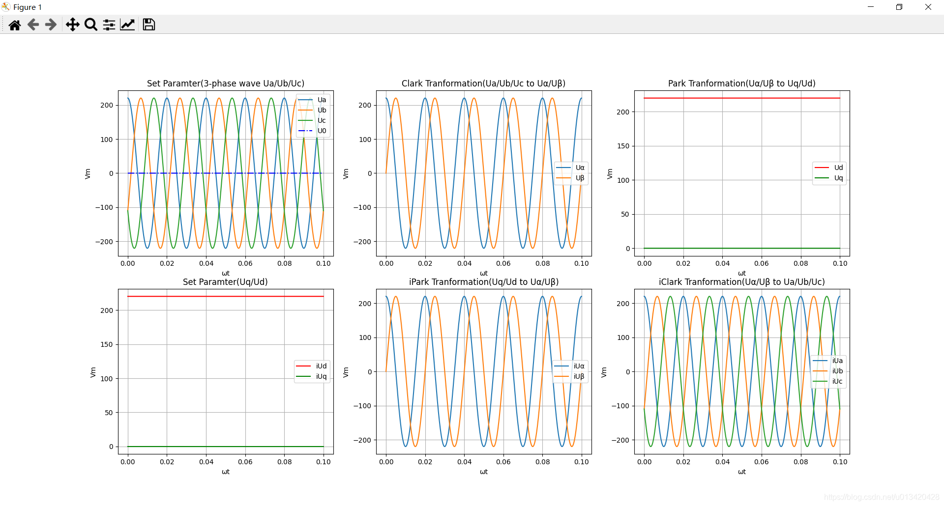
Python matplotlib仿真代码:

import numpy as np
import scipy as sp
import matplotlib.pyplot as plt
import matplotlib.pylab as plb


# 三相交流波形
Vm = 220    #电压幅度V
fHz=50      #频率
T=1/fHz     #周期
Tn = 5      #显示n个周期的波形

t = np.linspace(0, T*Tn, 360*Tn)    #时间t
theta = (2*np.pi*fHz) * t           #电相角θ=2πf,随时间变化θ=ωt=2πf·t
Ua = Vm * np.cos((2*np.pi*fHz) * t)                 #U
Ub = Vm * np.cos((2*np.pi*fHz) * t - 2.0943)#(2/3)*np.pi)   #V
Uc = Vm * np.cos((2*np.pi*fHz) * t + 2.0943)#(2/3)*np.pi)   #W
# 
Uo = (Ua+Ub+Uc) # (Ua+Ub+Uc)=0

plt.subplot(2,3,1)
plt.title('3-phase wave')
plt.title('Set Paramter(3-phase wave Ua/Ub/Uc)')
plt.plot(t, Ua, label='Ua')
plt.plot(t, Ub, label='Ub')
plt.plot(t, Uc, label='Uc')
plt.plot(t, Uo, 'b-.',label='U0')
plt.xlabel('ωt')
plt.ylabel('Vm')
plt.grid()
plt.legend()


# clark转换波形:
m = 2/3             #恒幅值
#m = np.sqrt(2/3)   #恒功率
Ualpha = m * (Ua - (1/2)*Ub - (1/2)*Uc)             #Uα
Ubeta =  m * (np.sqrt(3)/2 * Ub - np.sqrt(3)/2*Uc)  #Uβ
#Ualpha = Ua
#Ubeta = (1/np.sqrt(3))*(Ua + 2*Ub)
plt.subplot(2,3,2)
plt.title('Clark Tranformation(Ua/Ub/Uc to Uα/Uβ)')
plt.plot(t, Ualpha, label='Uα')
plt.plot(t, Ubeta, label='Uβ')
plt.xlabel('ωt')
plt.ylabel('Vm')
plt.grid()
plt.legend()


# park转换波形:
Ud =  Ualpha*np.cos(theta) + Ubeta*np.sin(theta)
Uq = -Ualpha*np.sin(theta) + Ubeta*np.cos(theta)
plt.subplot(2,3,3)
plt.title('Park Tranformation(Uα/Uβ to Uq/Ud)')
plt.plot(t, Ud, 'r', label='Ud')
plt.plot(t, Uq, 'g', label='Uq')
plt.xlabel('ωt')
plt.ylabel('Vm')
plt.legend()
plt.grid()



# iPark
Udi = Ud-0  #调节幅度(电机的转速)
Uqi = Uq-0  #调节相位(电机的转矩)
# 
plt.subplot(2,3,4)
plt.title('Set Paramter(Uq/Ud)')
plt.plot(t, Udi, 'r', label='iUd')
plt.plot(t, Uqi, 'g', label='iUq')
plt.xlabel('ωt')
plt.ylabel('Vm')
plt.legend()
plt.grid()


Ualphai = Udi *np.cos(theta) - Uqi * np.sin(theta) 
Ubetai = Udi * np.sin(theta) + Uqi * np.cos(theta)
plt.subplot(2,3,5)
plt.title('iPark Tranformation(Uq/Ud to Uα/Uβ)')
plt.plot(t, Ualphai, label='iUα')
plt.plot(t, Ubetai, label='iUβ')
plt.xlabel('ωt')
plt.ylabel('Vm')
plt.legend()
plt.grid()

# iClark波形:
m = 1           #恒幅值
#m=np.sqrt(2/3) #恒功率
Uai = m * (Ualphai +(0*Ubetai))
Ubi = m * (-(1/2)*Ualphai + (np.sqrt(3)/2)*Ubetai)
Uci = m * (-(1/2)*Ualphai - (np.sqrt(3)/2)*Ubetai)

plt.subplot(2,3,6)
plt.title('iClark Tranformation(Uα/Uβ to Ua/Ub/Uc)')
plt.plot(t, Uai, label='iUa')
plt.plot(t, Ubi, label='iUb')
plt.plot(t, Uci, label='iUc')
plt.xlabel('ωt')
plt.ylabel('Vm')
plt.legend()
plt.grid()

# 显示图像
plt.show()

仿真波形：