隐式神经表示二：超分网络学习傅里叶系数Local Texture Estimator for Implicit Representation Function

1. Local Texture Estimator for Implicit Representation Function

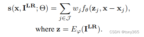
1. 通过隐式神经网络表示方法 实现 超分辨率。

一个典型的隐式表示方法作超分：

$z$ 是encoder的输出，可以理解为提取的图像特征
$x$ 是输入的坐标点映射到LR图像中，浮点类型， $x_j$ 是周围的4个点
$f_{\theta }$ 是解码器，本文解码器是一个MLP

可以理解为，输入一个坐标，利用 1）最近的4个点的特征$z_j$ 和 2）与最近4个点的 距离 $x-x_j$
得到解码后的值，进行双线性插值。如下图所示

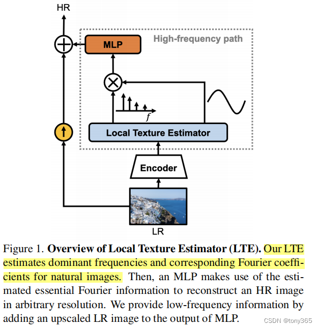
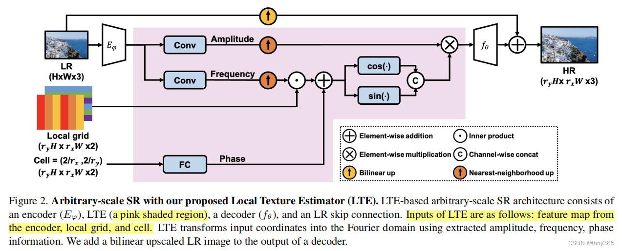
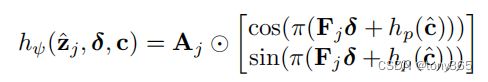
2. 在编码器和解码器之间作者引入一个 local texture estimator

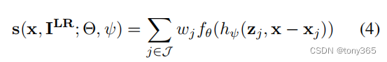
因此公式变为

$h_{\phi }$ 表示局部纹理估计，下图红色区域看起来复杂
其实就是下面的公式 其中 $ F, A, h_p©$ 分别表示 幅度，频率，相位
其中相位的输入是网格的长度 cell size

3. 代码分析

整体框架

    def forward(self, inp, coord, cell):
        self.gen_feat(inp)  # 生成特征
        return self.query_rgb(coord, cell) # 检索值

生成图像特征，编码器是一个常规的卷积网络，文中使用esdr,rdn, swinIR 等

feat 各通过一个卷积得到 coeff, freqq ,即幅度和频率

    def gen_feat(self, inp):
        self.inp = inp
        self.feat_coord = make_coord(inp.shape[-2:], flatten=False).cuda() \
            .permute(2, 0, 1) \
            .unsqueeze(0).expand(inp.shape[0], 2, *inp.shape[-2:])
        
        self.feat = self.encoder(inp)
        self.coeff = self.coef(self.feat)
        self.freqq = self.freq(self.feat)
        return self.feat

local texture estimator

首先根据输入的坐标 找到 最近邻的4个坐标，利用了循环，目的是求
$x-x_j$

vx_lst = [-1, 1]
vy_lst = [-1, 1]
eps_shift = 1e-6 

# field radius (global: [-1, 1])
rx = 2 / feat.shape[-2] / 2
ry = 2 / feat.shape[-1] / 2
for vx in vx_lst:
    for vy in vy_lst: # 周围的4个像素
        # prepare coefficient & frequency
        coord_ = coord.clone()
        coord_[:, :, 0] += vx * rx + eps_shift
        coord_[:, :, 1] += vy * ry + eps_shift
        coord_.clamp_(-1 + 1e-6, 1 - 1e-6)

接下来，就是根据 幅度，频率，相位得到 傅里叶表示，后续会输入 解码器
代码实现下面的公式

q_coef = F.grid_sample(
        coef, coord_.flip(-1).unsqueeze(1),
        mode='nearest', align_corners=False)[:, :, 0, :] \
        .permute(0, 2, 1)
q_freq = F.grid_sample(
    freq, coord_.flip(-1).unsqueeze(1),
    mode='nearest', align_corners=False)[:, :, 0, :] \
    .permute(0, 2, 1)
q_coord = F.grid_sample(
    feat_coord, coord_.flip(-1).unsqueeze(1),
    mode='nearest', align_corners=False)[:, :, 0, :] \
    .permute(0, 2, 1)
rel_coord = coord - q_coord # x - xj
rel_coord[:, :, 0] *= feat.shape[-2]
rel_coord[:, :, 1] *= feat.shape[-1]

# prepare cell
rel_cell = cell.clone()
rel_cell[:, :, 0] *= feat.shape[-2]
rel_cell[:, :, 1] *= feat.shape[-1]

# basis generation
bs, q = coord.shape[:2]
q_freq = torch.stack(torch.split(q_freq, 2, dim=-1), dim=-1)
q_freq = torch.mul(q_freq, rel_coord.unsqueeze(-1))
q_freq = torch.sum(q_freq, dim=-2)
q_freq += self.phase(rel_cell.view((bs * q, -1))).view(bs, q, -1)
q_freq = torch.cat((torch.cos(np.pi*q_freq), torch.sin(np.pi*q_freq)), dim=-1)

inp = torch.mul(q_coef, q_freq)            

接下来解码器是一个mlp网络

pred = self.imnet(inp.contiguous().view(bs * q, -1)).view(bs, q, -1)

双线性插值得到网络的结果， areas是双线性插值的系数

for pred, area in zip(preds, areas):
    ret = ret + pred * (area / tot_area).unsqueeze(-1)
        

将上面的结果，与双线性插值的 upscale LR 相加, 得到最后的结果，因此解码器输出的可以当作是
对低质量上采样的一个优化。

ret += F.grid_sample(self.inp, coord.flip(-1).unsqueeze(1), mode='bilinear',\
                      padding_mode='border', align_corners=False)[:, :, 0, :] \
                      .permute(0, 2, 1)

4. 网络数据的准备，网络的输入

利用下采样的得到 LR 图像

@register('sr-implicit-downsampled')
class SRImplicitDownsampled(Dataset):

    def __init__(self, dataset, inp_size=None, scale_min=1, scale_max=None,
                 augment=False, sample_q=None):
        self.dataset = dataset
        self.inp_size = inp_size
        self.scale_min = scale_min
        if scale_max is None:
            scale_max = scale_min
        self.scale_max = scale_max
        self.augment = augment
        self.sample_q = sample_q

    def __len__(self):
        return len(self.dataset)

    def __getitem__(self, idx):
        img = self.dataset[idx]
        s = random.uniform(self.scale_min, self.scale_max)

        if self.inp_size is None:
            h_lr = math.floor(img.shape[-2] / s + 1e-9)
            w_lr = math.floor(img.shape[-1] / s + 1e-9)
            img = img[:, :round(h_lr * s), :round(w_lr * s)] # assume round int
            img_down = resize_fn(img, (h_lr, w_lr))
            crop_lr, crop_hr = img_down, img
        else:
            w_lr = self.inp_size
            w_hr = round(w_lr * s)
            x0 = random.randint(0, img.shape[-2] - w_hr)
            y0 = random.randint(0, img.shape[-1] - w_hr)
            crop_hr = img[:, x0: x0 + w_hr, y0: y0 + w_hr]
            crop_lr = resize_fn(crop_hr, w_lr)

        if self.augment:
            hflip = random.random() < 0.5
            vflip = random.random() < 0.5
            dflip = random.random() < 0.5

            def augment(x):
                if hflip:
                    x = x.flip(-2)
                if vflip:
                    x = x.flip(-1)
                if dflip:
                    x = x.transpose(-2, -1)
                return x

            crop_lr = augment(crop_lr)
            crop_hr = augment(crop_hr)

        hr_coord, hr_rgb = to_pixel_samples(crop_hr.contiguous())

        if self.sample_q is not None:
            sample_lst = np.random.choice(
                len(hr_coord), self.sample_q, replace=False)
            hr_coord = hr_coord[sample_lst]
            hr_rgb = hr_rgb[sample_lst]

        cell = torch.ones_like(hr_coord)
        cell[:, 0] *= 2 / crop_hr.shape[-2]
        cell[:, 1] *= 2 / crop_hr.shape[-1]

        return {
            'inp': crop_lr,
            'coord': hr_coord,
            'cell': cell,
            'gt': hr_rgb
        }

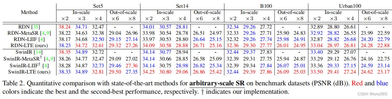
5. 结果

主要与meta-SR 和 LIIF进行比较，结果如下：

6. 相关文章做warp :

Learning Local Implicit Fourier Representation for Image Warping