ceres库学习

最新推荐文章于 2024-04-25 16:59:43 发布

我想静静，

最新推荐文章于 2024-04-25 16:59:43 发布

阅读量2.6k

点赞数 5

分类专栏： ceres 文章标签： ceres slam

本文链接：https://blog.csdn.net/weixin_42764932/article/details/118486779

版权

ceres 专栏收录该内容

3 篇文章 0 订阅

订阅专栏

ceres学习

功能
hello world
鲍威尔函数优化

ceres官方文档

功能

Ceres 可以解决以下形式的边界约束鲁棒化非线性最小二乘问题
在这里插入图片描述
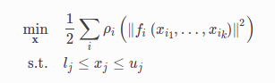
其中， $ρ_i(||f_i(x_{i_1},..., x_{i_k})||^2)$ 被称为ResidualBlock； $x_{i_1},..., x_{i_k}]$ 称为ParameterBlock；
$l_j$ 和 $u_j$ 是参数块的边界， $ρ_i$ 是一个LossFunction, LossFunction是标量函数，用于减少异常值对非线性最小二乘问题的解决方案的影响，通常为衡等变换.

hello world

待优化问题：
在这里插入图片描述
评估函数CostFunction为 $f (x) = 10 - x$

ceres求解步骤

定义CostFuntion，通过函数重载运算操作符定义代价函数，就是形式里面的f(x)
构建Problem，设置代价函数，AutoDiffCostFunction将刚刚建立的CostFunctor 结构的一个实例作为输入，自动生成其微分并且赋予其一个CostFunction 类型的接口。调用AddResidualBlock将误差添加到目标函数中，由于优化需要梯度，我们有三种选择：
1）使用Ceres自带的自动求导（Auto Diff）
2）使用数值求导（Numeric Diff）
3）使用自己求导的解析求导形式，提供给ceres。
配置Solver，在options里可以配置各种优化的选项，可以选择Line Search或者Trust Region、迭代次数、步长等等
定义Summary
开始优化Solve
输出结果SUmmary.BriefReport

#include <iostream>
#include <ceres/ceres.h>
#include "glog/logging.h"

using ceres::AutoDiffCostFunction;
using ceres::CostFunction;
using ceres::Problem;
using ceres::Solve;
using ceres::Solver;

using namespace std;

//1. 定义CostFuntion
struct CostFunctor{
    template<typename T>
    bool operator()(const T* const x, T*residual)const{
        residual[0] = T(10.0) - x[0];
        return true;
    }
};


int main(int argc, char** argv) 
{
    //初始化
    double init_x = 5.0;
    double x = init_x;
    //2. 构建问题
    Problem problem;
	
	//设置目标函数，AutoDiffCostFunction将刚刚建立的CostFunctor 结构的一个实例作为输入，自动生成其微分并且赋予其一个CostFunction 类型的接口
    CostFunction* cost_function =
            new AutoDiffCostFunction<CostFunctor, 1, 1>(new CostFunctor);
   //添加误差项，调用AddResidualBlock将误差添加到目标函数中
    problem.AddResidualBlock(cost_function, nullptr, &x);

	//3. 调用solve函数求解，在options里可以配置各种优化的选项，可以选择Line Search或者Trust Region、迭代次数、步长等等
    Solver::Options options;
    options.minimizer_progress_to_stdout = true;
    
	//4. 定义Summary
    Solver::Summary summary;
    
    //5. 开始优化Solve
    Solve(options, &problem, &summary);
    
	//6.输出结果SUmmary.BriefReport
    cout<<summary.BriefReport()<<"\n";
    cout<<"x: "<<init_x<<" -> "<<x<<"\n";
    return 0;
}

cmakelist

cmake_minimum_required(VERSION 2.8)
project(p1)

set( CMAKE_BUILD_TYPE "Release" )
set( CMAKE_CXX_FLAGS "-O3" )

include_directories("/usr/include/eigen3")

find_package( Ceres REQUIRED )
include_directories( ${CERES_INCLUDE_DIRS} )


add_executable(p1 main.cpp)
target_link_libraries(p1 Ceres::ceres)

Ceres学习笔记之CMakeLists写法总结https://blog.csdn.net/sinat_28752257/article/details/82758546

跟我一起写Makefile

数值法求导（Numeric Derivatives）

在某些情况下，像在Hello World中一样定义一个代价函数是不可能的。比如在求解残差值（residual）的时候调用了一个库函数，而这个库函数的内部算法你根本无法干预。在这种情况下数值微分算法就派上用场了。用户定义一个CostFunctor来计算残差值，并且构建一个NumericDiffCostFunction数值微分代价函数。

Ceres官方更加推荐自动微分算法，因为C++模板类使自动算法有更高的效率。数值微分算法通常来说计算更复杂，收敛更缓慢。

比如对于 f(x)=10−x 对应函数体如下：

struct NumericDiffCostFunctor {
  bool operator()(const double* const x, double* residual) const {
    residual[0] = 10.0 - x[0];
    return true;
  }
  }
//struct CostFunctor {
//    template <typename T>
//    bool operator()(const T* const x, T* residual) const {
//        residual[0] = T(10.0) - x[0];
//        return true;
//    }
//};

可以发现，没用模板类。

然后继续添加Problem

CostFunction* cost_function =
  new NumericDiffCostFunction<NumericDiffCostFunctor, ceres::CENTRAL, 1, 1>(
      new NumericDiffCostFunctor);
problem.AddResidualBlock(cost_function, NULL, &x);

//    CostFunction* cost_function =
//            new AutoDiffCostFunction<CostFunctor, 1, 1>(new CostFunctor);
//    problem.AddResidualBlock(cost_function, NULL, &x);
//

在用Nummeric算法时需要额外给定一个参数ceres::CENTRAL ，这个参数告诉计算机如何计算导数。

ceres:: FORWARD

在这里插入图片描述

ceres::CENTRAL

在这里插入图片描述

ceres::RIDDERS

在这里插入图片述
注：随着步长h的下降，误差逐渐减小，但由于舍入误差，h进一步下降时，误差增大。

Central Differences 的成本大约是 Forward Differences 的两倍，并且 Ridders 方法的显着提高了准确性但运行时间增加了一个数量级。

解析法求导（Analytic Derivatives）

有些时候，应用自动求解算法时不可能的。比如在某些情况下，计算导数的时候，使用闭合解（closed form，也被称为解析解）会比使用自动微分算法中的链式法则（chain rule）更有效率。

解析解(analytical solution)：
就是一些严格的公式,给出任意的自变量就可以求出其因变量,也就是问题的解。他人可以利用这些公式计算各自的问题。所谓的解析解是一种包含：分式、三角函数、指数、对数甚至无限级数等基本函数的解的形式。对任一独立变量，我们皆可将其带入解析函数求得正确的相依变量。因此，解析解也被称为闭式解（closed-form solution）。

数值解(numerical solution)：是采用某种计算方法,如有限元的方法, 数值逼近,插值的方法得到的解。别人只能利用数值计算的结果,而不能随意给出自变量并求出计算值。此方法所求得的相依变量为一个个分离的数值。

提供您自己的残差和雅可比计算代码：

比如对于 f(x)=10−x

class QuadraticCostFunction : public ceres::SizedCostFunction<1, 1> {
 public:
  virtual ~QuadraticCostFunction() {}
  virtual bool Evaluate(double const* const* parameters,
                        double* residuals,
                        double** jacobians) const {
    const double x = parameters[0][0];
    residuals[0] = 10 - x;

    // Compute the Jacobian if asked for.
    if (jacobians != nullptr && jacobians[0] != nullptr) {
      jacobians[0][0] = -1;
    }
    return true;
  }
};

实现 CostFunction对象有点繁琐。我们建议除非您有充分的理由自己管理雅可比计算，否则您可以使用AutoDiffCostFunction或 NumericDiffCostFunction构建残差块。

添加problem

CostFunction* cost_function = new QuadraticCostFunction;
problem.AddResidualBlock(cost_function, NULL, &x);

整体代码

#include <iostream>
#include <ceres/ceres.h>
#include "glog/logging.h"

using ceres::AutoDiffCostFunction;
using ceres::NumericDiffCostFunction;
using ceres::CostFunction;
using ceres::Problem;
using ceres::Solve;
using ceres::Solver;

using namespace std;

class QuadraticCostFunction : public ceres::SizedCostFunction<1, 1> {
public:
    virtual ~QuadraticCostFunction() {}
    virtual bool Evaluate(double const* const* parameters,
                          double* residuals,
                          double** jacobians) const {
        const double x = parameters[0][0];
        residuals[0] = 10 - x;

        // Compute the Jacobian if asked for.
        if (jacobians != nullptr && jacobians[0] != nullptr) {
            jacobians[0][0] = -1;
        }
        return true;
    }
};


int main(int argc, char** argv) {
    double init_x = 5.0;
    double x = init_x;

    Problem problem;

    CostFunction* cost_function = new QuadraticCostFunction;
    problem.AddResidualBlock(cost_function, NULL, &x);

    Solver::Options options;
    options.minimizer_progress_to_stdout = true;
    Solver::Summary summary;
    Solve(options, &problem, &summary);

    cout<<summary.BriefReport()<<"\n";
    cout<<"x: "<<init_x<<" -> "<<x<<"\n";
    return 0;
}

其他

计算导数是迄今为止使用 Ceres 最复杂的部分，根据情况，用户可能需要更复杂的计算导数的方法。本节只是触及如何向 Ceres 提供Derivatives的皮毛。一旦你习惯使用 NumericDiffCostFunction，并AutoDiffCostFunction建议在考虑看看DynamicAutoDiffCostFunction， CostFunctionToFunctor，NumericDiffFunctor以及 ConditionedCostFunction构建和计算成本函数的更先进的方法。

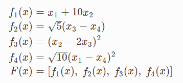
鲍威尔函数优化

在这里插入图片描述

#include <iostream>
#include <ceres/ceres.h>
#include "glog/logging.h"

using ceres::AutoDiffCostFunction;
using ceres::CostFunction;
using ceres::Problem;
using ceres::Solve;
using ceres::Solver;

using namespace std;

struct f1{
    template<typename T>
    bool operator()(const T* const x1, const T* const x2, T*residual)const{
        residual[0] = x1[0] + 10.0 * x2[0];
        return true;
    }
};
struct f2{
    template<typename T>
    bool operator()(const T* const x3, const T* const x4, T*residual)const{
        residual[0] = sqrt(5.0) * (x3[0] - x4[0]);
        return true;
    }
};
struct f3{
    template<typename T>
    bool operator()(const T* const x2, const T* const x3, T*residual)const{
        residual[0] = (x2[0] - 2.0 * x3[0]) * (x2[0] - 2.0 * x3[0]);
        return true;
    }
};
struct f4{
    template<typename T>
    bool operator()(const T* const x1, const T* const x4, T*residual)const{
        residual[0] = sqrt(10.0) * (x1[0] - x4[0]) * (x1[0] - x4[0]);
        return true;
    }
};

int main(int argc, char** argv) {
    double x1 = 3.0;
    double x2 = -1.0;
    double x3 = 0.0;
    double x4 = 1.0;

    Problem problem;

    problem.AddResidualBlock(
            new AutoDiffCostFunction<f1, 1, 1, 1>(new f1), nullptr, &x1, &x2);
    problem.AddResidualBlock(
            new AutoDiffCostFunction<f2, 1, 1, 1>(new f2), nullptr, &x3, &x4);
    problem.AddResidualBlock(
            new AutoDiffCostFunction<f3, 1, 1, 1>(new f3), nullptr, &x2, &x3);
    problem.AddResidualBlock(
            new AutoDiffCostFunction<f4, 1, 1, 1>(new f4), nullptr, &x1, &x4);

    Solver::Options options;
    options.max_num_iterations = 100;
    options.linear_solver_type = ceres::DENSE_QR;
    options.minimizer_progress_to_stdout = true;

    std::cout << "Initial x1 = " << x1
              << ", x2 = " << x2
              << ", x3 = " << x3
              << ", x4 = " << x4
              << "\n";

    Solver::Summary summary;
    Solve(options, &problem, &summary);

    cout<<summary.BriefReport()<<"\n";
    std::cout << "Final x1 = " << x1
              << ", x2 = " << x2
              << ", x3 = " << x3
              << ", x4 = " << x4
              << "\n";
    return 0;
}

我想静静，

关注

5
点赞
踩
20

收藏

觉得还不错? 一键收藏
3
评论
ceres库学习

ceres学习功能hello world数值法求导（Numeric Derivatives）ceres:: FORWARDceres::CENTRALceres::RIDDERS解析法求导（Analytic Derivatives）其他鲍威尔函数优化ceres官方文档功能Ceres 可以解决以下形式的边界约束鲁棒化非线性最小二乘问题其中，ρi(∣∣fi(xi1,...,xik)∣∣2)ρ_i(||f_i(x_{i_1},..., x_{i_k})||^2)ρi(∣∣fi(xi1,...,x
复制链接

扫一扫