全局坐标系与车身坐标系转换

穿越临界点

已于 2022-08-10 23:57:41 修改

阅读量6.5k

点赞数 18

分类专栏：自动驾驶文章标签：人工智能自动驾驶

于 2022-08-10 23:44:05 首次发布

本文链接：https://blog.csdn.net/weixin_44873133/article/details/126276413

版权

自动驾驶专栏收录该内容

13 篇文章 36 订阅

订阅专栏

在学习资料满天飞的大环境下，知识变得非常零散，体系化的知识并不多，这就导致很多人每天都努力学习到感动自己，最终却收效甚微，甚至放弃学习。我的使命就是过滤掉大量的无效信息，将知识体系化，以短平快的方式直达问题本质，把大家从大海捞针的痛苦中解脱出来。

文章目录

0 前言

做规划控制必然离不开坐标和坐标变换。一般涉及到的就是全局坐标系和车身坐标系互转，还有笛卡尔坐标系和自然坐标系之间的转换。坐标转换一般会涉及到三角函数、向量、复数、矩阵等知识。

本篇先介绍全局坐标系与车身坐标系之间的转换，为后续的内容热一下身。

1 全局坐标系和车身坐标系

1.1 全局坐标系

一般全局坐标系是将地球作为参考系进行定义的，也就是大地坐标系。

对于行车来说，车辆在大地上的位置信息通常来自于卫星导航系统，位置坐标在WGS-84坐标系（地理坐标系，使用经纬度表示任意位置）中表示。为了方便计算距离和面积，还需要通过通用横轴墨卡托（Universal Transverse Mercator, UTM）网络系统将其转换至笛卡尔坐标系。

但对于局部泊车系统来说，不需要全局定位，也就无需考虑地理坐标系因素，只需要在地图上选取一点作为原点构建全局坐标系即可。

1.2 车身坐标系

车身坐标系是将车辆自身作为参考系建立的坐标系。原点一般选取车辆后轴中心点或者车辆的质心。

车辆上安装的各种传感器（比如摄像头、雷达）的位置，以及车辆的轮廓（如果是用矩形逼近车辆轮廓，则通常使用四个角点表示车辆轮廓）都需要使用车身坐标系下的坐标。

2 坐标系转换

2.1 旋转矩阵推导

2.1.1 坐标变换和向量旋转的关系

一个向量 $\overrightarrow{OP}$ 旋转 $\theta$ 角度，相当于先把坐标系A旋转 $\theta$ 角度得到坐标系B，然后在坐标系B中取与 $\overrightarrow{OP}$ 相同坐标值的向量 $\overrightarrow{OQ}$ ，最后再把 $\overrightarrow{OQ}$ 的坐标映射回坐标系A。

相应地，将坐标系B（相对于坐标系A的夹角为 $\theta$ ）中的一个坐标值映射到坐标系A的操作就等同于——在坐标系A中先取和坐标系B中相同坐标值的向量，然后将其旋转 $\theta$ 角度。

为什么会有这种等价关系呢？

因为坐标和向量是等价的，坐标只是向量的一种表示方法。坐标系和向量空间也是等价的，坐标轴就是相互正交的单位向量，对坐标轴的操作等价于/可以代替对整个向量空间中向量的操作。

Tips：对概念的深入理解很重要，尤其是等价变换。因为这往往是公式推导和证明的思路。

2.1.2 基于复数和欧拉公式推导

在复平面上使用复数乘法等价向量旋转运算。
$\begin{align} \overrightarrow{OQ} &= \overrightarrow{OP} \cdot e^{i\theta} \\[2ex] &=(x_p+iy_p) \cdot (cos\theta + isin\theta)\\[2ex] &=(cos\theta \cdot x_p - sin\theta \cdot y_p) + i(sin\theta \cdot x_p + cos\theta \cdot y_p) \end{align} \tag 1$
易得：
$\begin{aligned} \left[ \begin{array}{cc} x_{q} \\ y_{q} \end{array} \right ] &= \left[ \begin{array}{cc} cos\theta,& -sin\theta \\ sin\theta,& cos\theta \\ \end{array} \right ] \cdot \left[ \begin{array}{cc} x_{p} \\ y_{p} \\ \end{array} \right ]\\[3ex] &=R \cdot \left[ \begin{array}{cc} x_{p} \\ y_{p} \\ \end{array} \right ] \end{aligned} \tag2$
其中， $R$ 即为旋转矩阵。

2.1.3 基于纯向量运算推导

在这里插入图片描述

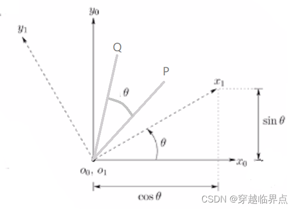
如图所示，坐标系B( $x_1o_1y_1$ ) 相对于坐标系A( $x_0o_0y_0$ ) 旋转了 $\theta$ 角度。两个坐标系内的任意两个坐标值相同（指在各自坐标系中的坐标值）的两个向量均相差 $\theta$ 角度。

所以，求坐标系B中的某一坐标值（向量）在坐标系A中的坐标值（向量投影），就等价于求坐标系B的坐标轴（基底）在坐标系A上的坐标值（投影）。

则有
$\begin{align} R &= [X_1^0, Y_1^0] \\[3ex] &= \left[ \begin{array}{cc} x_1 \cdot x_0,& y_1 \cdot x_0 \\ x_1 \cdot y_0,& y_1 \cdot y_0 \\ \end{array} \right ] \\[3ex] &= \left[ \begin{array}{cc} cos\theta,& cos(\frac{\pi}{2}+\theta) \\ sin\theta,& sin(\frac{\pi}{2}+\theta) \\ \end{array} \right ]\\[3ex] &= \left[ \begin{array}{cc} cos\theta,& -sin\theta \\ sin\theta,& cos\theta \\ \end{array} \right ] \end{align}\tag3$

2.2 车身坐标系转全局坐标系

以二维平面为例。设 $[x_v,y_v,\theta_v]$ 为车辆在当前位置的全局位姿；设 $[x_r,y_r,\theta_r]$ 为传感器Sensor相对于车身的位姿；设 $[x_s,y_s,\theta_s]$ 为传感器Sensor的全局位姿。

车身坐标系对应前文中的坐标系B，全局坐标系对应前文中的坐标系A。

对坐标进行旋转加平移变换，则有：
$\theta_s = \theta_v + \theta_r \\[3ex] \begin{aligned} \left[ \begin{array}{} x_{s} \\ y_{s} \\ \end{array} \right ] &= \left[ \begin{array}{cc} cos\theta_v,& -sin\theta_v \\ sin\theta_v,& cos\theta_v \\ \end{array} \right ] \cdot \left[ \begin{array}{cc} x_{r} \\ y_{r} \\ \end{array} \right ]+ \left[ \begin{array}{cc} x_{v} \\ y_{v} \\ \end{array} \right] \end{aligned} \tag4$

2.3 全局坐标系转车身坐标系

对旋转矩阵求逆可以得到：
$R^{-1} = R^*/1= \left[ \begin{array}{} cos\theta_v, & sin\theta_v \\ -sin\theta_v, & cos\theta_v \\ \end{array} \right] \tag5$
从而可以推得：

$\theta_r = \theta_s - \theta_v \\[3ex] \begin{aligned} \left[ \begin{array}{cc} x_{r} \\ y_{r} \\ \end{array} \right ] &= \left[ \begin{array}{cc} cos\theta_v,& sin\theta_v \\ -sin\theta_v,& cos\theta_v \\ \end{array} \right ] \cdot \left[ \begin{array}{cc} x_{s}-x_v \\ y_{s}-x_v \\ \end{array} \right ] \end{aligned} \tag6$